1 Introduction to Geology
What is Geology?
In its broadest sense, geology is the study of Earth—its interior and its exterior surface, the minerals, rocks and other materials that are around us, the processes that have resulted in the formation of those materials, the water that flows over the surface and through the ground, the changes that have taken place over the vastness of geological time, and the changes that we can anticipate will take place in the near future. Geology is a science, meaning that we use deductive reasoning and scientific methods to understand geological problems. It is, arguably, the most integrated of all of the sciences because it involves the understanding and application of all of the other sciences: physics, chemistry, biology, mathematics, astronomy, and others. But unlike most of the other sciences, geology has an extra dimension, that of time—deep time—billions of years of it. Geologists study the evidence that they see around them, but in most cases, they are observing the results of processes that happened thousands, millions, and even billions of years in the past. Those were processes that took place at incredibly slow rates—millimetres per year to centimetres per year—but because of the amount of time available, they produced massive results.
Geology is also about understanding the evolution of life on Earth; about discovering resources such as water, metals and energy; about recognizing and minimizing the environmental implications of our use of those resources; and about learning how to mitigate the hazards related to earthquakes, volcanic eruptions, and slope failures.
What are scientific methods?
There is no single method of inquiry that is specifically the “scientific method”; furthermore, scientific inquiry is not necessarily different from serious research in other disciplines. The most important thing that those involved in any type of inquiry must do is to be skeptical. As the physicist Richard Feynman once said: the first principle of science is that “you must not fool yourself—and you are the easiest person to fool.” A key feature of serious inquiry is the creation of a hypothesis (a tentative explanation) that could explain the observations that have been made, and then the formulation and testing (by experimentation) of one or more predictions that follow from that hypothesis.
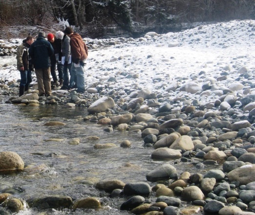
For example, we might observe that most of the cobbles in a stream bed are well rounded (see Figure 1.1.2), and then derive the hypothesis that the rocks are rounded by transportation along the stream bed. A prediction that follows from this hypothesis is that cobbles present in a stream will become increasingly rounded as they are transported downstream. An experiment to test this prediction would be to place some angular cobbles in a stream, label them so that we can be sure to find them again later, and then return at various time intervals (over a period of years) to carefully measure their locations and roundness.
A critical feature of a good hypothesis and any resulting predictions is that they must be testable. For example, an alternative hypothesis to the one above is that an extraterrestrial organization creates rounded cobbles and places them in streams when nobody is looking. This may indeed be the case, but there is no practical way to test this hypothesis. Most importantly, there is no way to prove that it is false, because if we aren’t able to catch the aliens at work, we still won’t know if they did it!
Minerals and Rocks
The Earth is made up of varying proportions of the 90 naturally occurring elements—hydrogen, carbon, oxygen, magnesium, silicon, iron, and so on. In most geological materials, these combine in various ways to make minerals.
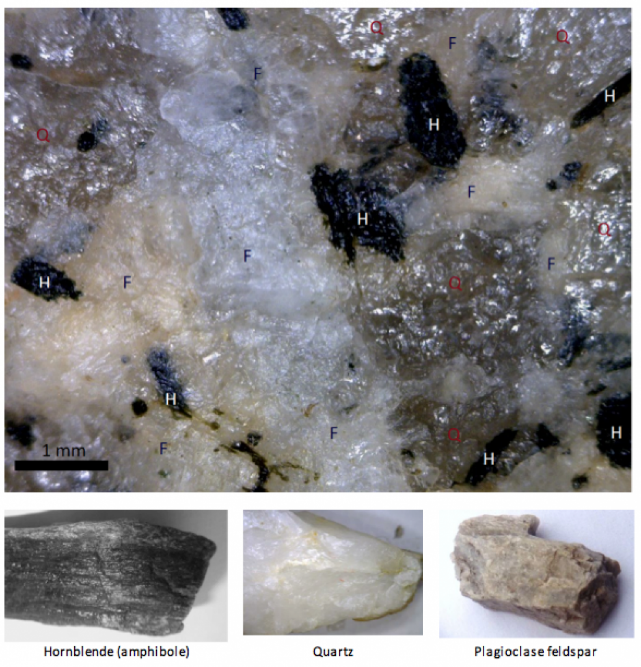
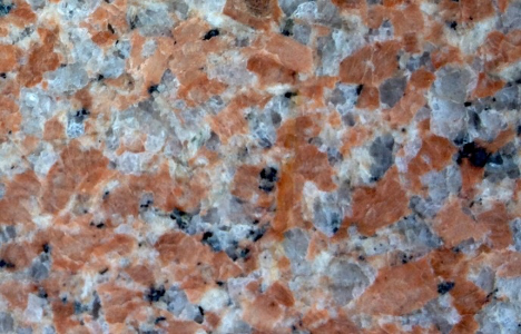
A mineral is a naturally occurring combination of specific elements that are arranged in a particular repeating three-dimensional structure or lattice. There are thousands of minerals. In nature, minerals are found in rocks, and the vast majority of rocks are composed of at least a few different minerals. A close-up view of granite, a common rock, is shown in Figure 1.4.2. Although a hand-sized piece of granite may have thousands of individual mineral crystals in it, there are typically only a few different minerals, as shown here.
Rocks can form in a variety of ways. Igneous rocks form from magma (molten rock) that has either cooled slowly underground (e.g., to produce granite) or cooled quickly at the surface after a volcanic eruption (e.g. basalt). Sedimentary rocks, such as sandstone, form when the weathered products of other rocks accumulate at the surface and are then buried by other sediments. Metamorphic rocks form when either igneous or sedimentary rocks are heated and squeezed to the point where some of their minerals are unstable and new minerals form to create a different type of rock. An example is schist.
A critical point to remember is the difference between a mineral and a rock. A mineral is a pure substance with a specific composition and structure, while a rock is typically a mixture of several different minerals (although a few types of rock may include only one type of mineral). Examples of minerals are feldspar, quartz, mica, halite, calcite, and amphibole. Examples of rocks are granite, basalt, sandstone, limestone, and schist.
The Rock Cycle
The rock components of the crust are slowly but constantly being changed from one form to another and the processes involved are summarized in the rock cycle (Figure 3.1.1). The rock cycle is driven by two forces: (1) Earth’s internal heat engine, which moves material around in the core and the mantle and leads to slow but significant changes within the crust, and (2) the hydrological cycle, which is the movement of water, ice, and air at the surface, and is powered by the sun.
The rock cycle is still active on Earth because our core is hot enough to keep the mantle moving, our atmosphere is relatively thick, and we have liquid water. On some other planets or their satellites, such as the Moon, the rock cycle is virtually dead because the core is no longer hot enough to drive mantle convection and there is no atmosphere or liquid water.
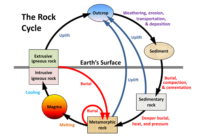
In describing the rock cycle, we can start anywhere we like, although it’s convenient to start with magma. As we’ll see in more detail below, magma is rock that is hot to the point of being entirely molten, with a temperature of between about 800° and 1300°C, depending on the composition and the pressure.
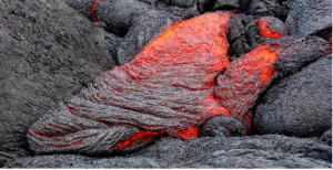
Magma can either cool slowly within the crust (over centuries to millions of years)—forming intrusive igneous rock, or erupt onto the surface and cool quickly (within seconds to years)—forming extrusive igneous rock (volcanic rock) (Figure 3.1.2). Intrusive igneous rock typically crystallizes at depths of hundreds of metres to tens of kilometres below the surface. To change its position in the rock cycle, intrusive igneous rock has to be uplifted and then exposed by the erosion of the overlying rocks.
Through the various plate-tectonics-related processes of mountain building, all types of rocks are uplifted and exposed at the surface. Once exposed, they are weathered, both physically (by mechanical breaking of the rock) and chemically (by weathering of the minerals), and the weathering products—mostly small rock and mineral fragments—are eroded, transported, and then deposited as sediments. Transportation and deposition occur through the action of glaciers, streams, waves, wind, and other agents, and sediments are deposited in rivers, lakes, deserts, and the ocean.
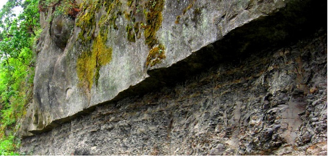
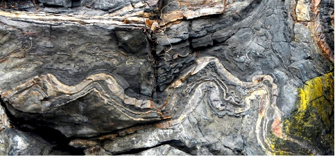
Unless they are re-eroded and moved along, sediments will eventually be buried by more sediments. At depths of hundreds of metres or more, they become compressed and cemented into sedimentary rock (See Figure 3.1.3 for example). Again through various means, largely resulting from plate-tectonic forces, different kinds of rocks are either uplifted, to be re-eroded, or buried deeper within the crust where they are heated up, squeezed, and changed into metamorphic rock (Figure 3.1.4)
Fundamentals of Plate Tectonics
Plate Tectonics is the model or theory that has been used for the past 60 years to understand and explain how the Earth works—more specifically the origins of continents and oceans, of folded rocks and mountain ranges, of earthquakes and volcanoes, and of continental drift.
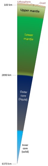
Key to understanding plate tectonics is an understanding of Earth’s internal structure, which is illustrated in Figure 1.5.1. Earth’s core consists mostly of iron. The outer core is hot enough for the iron to be liquid. The inner core—although even hotter—is under so much pressure that it is solid. The mantle is made up of iron and magnesium minerals. The bulk of the mantle surrounding the outer core is solid rock, but is plastic enough to be able to flow slowly. The outermost part of the mantle is rigid. The crust —composed mostly of granite on the continents and mostly of basalt beneath the oceans—is also rigid. The crust and outermost rigid mantle together make up the lithosphere. The lithosphere is divided into about 20 tectonic plates that move in different directions on Earth’s surface.
An important property of Earth (and other planets) is that the temperature increases with depth, from close to 0°C at the surface to about 7000°C at the centre of the core. In the crust, the rate of temperature increase is about 30°C every kilometre. This is known as the geothermal gradient.
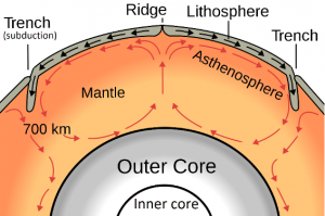
Heat is continuously flowing outward from Earth’s interior, and the transfer of heat from the core to the mantle causes convection in the mantle (Figure 1.5.2). This convection is the primary driving force for the movement of tectonic plates. At places where convection currents in the mantle are moving upward, new lithosphere forms (at ocean ridges), and the plates move apart (diverge). Where two plates are converging (and the convective flow is downward), one plate will be subducted (pushed down) into the mantle beneath the other. Many of Earth’s major earthquakes and volcanoes are associated with convergent boundaries.
Plates, Plate Motions, and Plate Boundary Processes
Alfred Wegener (1880-1930) earned a PhD in astronomy at the University of Berlin in 1904, but he had always been interested in geophysics and meteorology and spent most of his academic career working in meteorology. In 1911 he happened on a scientific publication that included a description of the existence of matching Permian-aged terrestrial fossils in various parts of South America, Africa, India, Antarctica, and Australia (Figure 10.1.2).
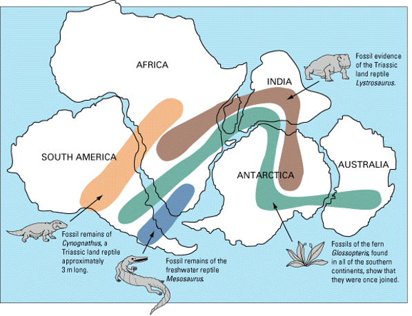
Wegener concluded that this distribution of terrestrial organisms could only exist if these continents were joined together during the Permian, and he coined the term Pangea (“all land”) for the supercontinent that he thought included all of the present-day continents.
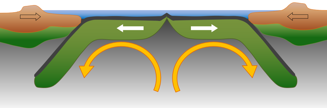
In 1960, Harold Hess, a widely respected geologist from Princeton University, advanced a theory with many of the elements that we now accept as plate tectonics. Hess proposed that new sea floor was generated from mantle material at the ocean ridges, and that old sea floor was dragged down at the ocean trenches and re-incorporated into the mantle. He suggested that the process was driven by mantle convection currents, rising at the ridges and descending at the trenches (Figure 10.3.8). He also suggested that the less-dense continental crust did not descend with oceanic crust into trenches, but that colliding land masses were thrust up to form mountains. Hess’s theory formed the basis for our ideas on sea-floor spreading and continental drift, but it did not deal with the concept that the crust is made up of specific plates. Although the Hess model was not roundly criticized, it was not widely accepted (especially in the U.S.), partly because it was not well supported by hard evidence.
Continental drift and seafloor spreading became widely accepted around 1965 as more and more data became available and geologists started thinking in these terms. By the end of 1967 the Earth’s surface had been mapped into a series of plates (Figure 10.4.1). The major plates are Eurasia, Pacific, India, Australia, North America, South America, Africa, and Antarctic. There are also numerous small plates (e.g., Juan de Fuca, Cocos, Nazca, Scotia, Philippine, Caribbean), and many very small plates or sub-plates. For example, the Juan de Fuca Plate is actually three separate plates (Gorda, Juan de Fuca, and Explorer) that all move in the same general direction but at slightly different rates.
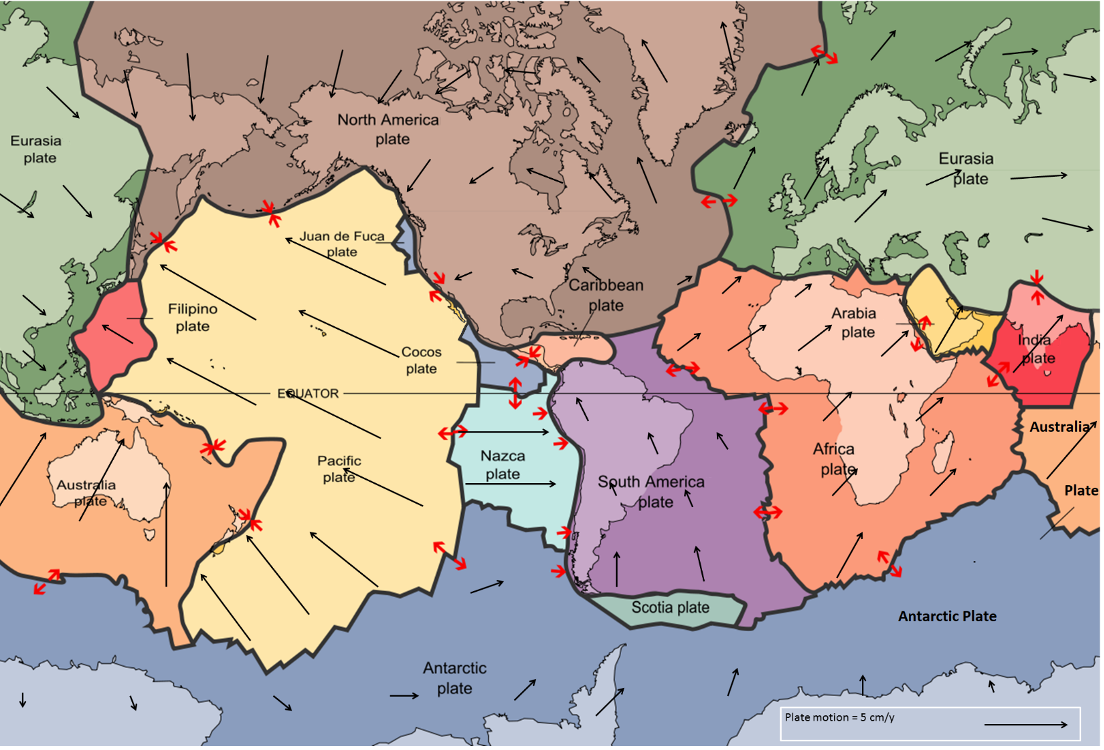
Figure 10.4.1 image description: Descriptions of 15 different plates and their movements
|
Plate name |
Description of plate |
Bordering plates (ordered from longest border to shortest) |
Description of movement |
|---|---|---|---|
|
Africa plate |
This plate includes all of Africa and the surrounding ocean, including the eastern Atlantic Ocean, the surrounding Antarctic Ocean, and the western Indian ocean. |
South America plate, Antarctic plate, Eurasia plate, North America plate, Arabia plate, India plate, Australia plate |
This plate is moving north east towards the Arabia and Eurasia plates. |
|
Antarctic plate. |
This plate makes up all of Antarctica and much of the surrounding ocean. |
Pacific plate, Australia plate, Africa plate, Scotia plate, Nazca plate, South America plate. |
The part of the plate around the South America plate is moving northwards and a little east. The part of the plate around the Australia plate is moving southwards. |
|
Arabia plate |
This plate includes all of Saudi Arabia, and much of the Levant (up to Iraq and Syria). |
Eurasia plate, Africa plate, India plate |
This plate is moving north east towards the Eurasia plate. |
|
Australia plate |
This plate includes Australia and much of the surrounding ocean. New Guinea and the northern parts of New Zealand are part of the Australia plate. The ocean area along southern Asia up to the India plate is also a part of the Australia plate. |
Antarctic plate, Pacific plate, Eurasia plate, India Plate, Africa plate. |
This plate is moving north east towards the Eurasia plate and the Pacific plate. |
|
Caribbean plate |
This plate is small. It includes the central Caribbean countries and runs along the northern edge of South America. |
North America plate, South America plate, Cocos plate. |
N/A |
|
Cocos plate |
This plate is small. It runs along the west coast of Mexico and western Caribbean countries. |
Nazca plate, Pacific plate, North America plate, Caribbean plate. |
This plate is moving north east towards the Caribbean and North America plates. |
|
Eurasia plate |
This plate includes the northeastern part of the Atlantic Ocean, all of Europe, all of Russia (except its most eastern part), and down through southeast Asia, including China and Indonesia. |
North America plate, Africa plate, Australia plate, Arabia plate, India plate, Filipino plate. |
This plate is rotating in a clockwise direction towards the Pacific plate. |
|
Filipino plate |
This plate includes the islands that make up the Philippines and north to include parts of southern Japan. |
Eurasia plate, Pacific plate. |
This plate is moving north west towards the Eurasia plate. |
|
India plate |
This plate includes India and the surrounding India Ocean. |
Australia plate, Eurasia plate, Africa plate, Arabia plate. |
This plate is moving north-north east towards the Eurasia plate. |
|
Juan de Fuca plate |
This plate is small. It runs along the north western coast of the United States and the southern British Columbia coast. |
Pacific plate, North America plate. |
N/A |
|
Nazca plate |
This plate is in the Pacific Ocean between the Pacific plate and the South America plate. |
South America plate, Pacific plate, Antarctic plate, Cocos plate |
This plate is moving directly east towards the South America plate. |
|
North America Plate |
This plate includes all of North America, Greenland, the eastern most part of Russia, northern Japan, and the northwestern part of the Atlantic Ocean. |
Eurasia plate, Pacific plate, Africa plate, Caribbean plate, South America plate, Cocos plate, Juan de Fuca plate |
This plate is rotating counter clockwise in towards the Pacific plate. |
|
Pacific plate |
This plate makes up most of the Pacific Ocean. |
North America plate, Australia plate, Antarctic plate, Nazca plate, Filipino plate, Cocos plate, Juan de Fuca plate |
This plate is moving northwest towards the Australia, Filipino, and Eurasia plates. |
|
Scotia plate |
This plate is small. It runs from the tip of South America eastwards to form a barrier between the Antarctic plate and the South America plate. |
Antarctic plate, South America plate. |
N/A |
|
South America plate |
This plate starts at the western edge of South America and stretches east into the southwestern parst of the Atlantic Ocean. |
Africa plate, Nazca plate, Scotia plate, Caribbean plate, Antarctic plate, North America plate |
This plate moves north and slightly west towards the Caribbean plate and the North America plate. |
Check out how Earth’s tectonic plates have moved over the past 200 million years: Continents collide and break apart over time (2:09).
Want to see how things have changed closer to home? Check out How North American got its Shape (4:58).
Rates of motions of the major plates range from less than 1 cm/y to over 10 cm/y. The Pacific Plate is the fastest, followed by the Australian and Nazca Plates. The North American Plate is one of the slowest, averaging around 1 cm/y in the south up to almost 4 cm/y in the north.
Plates move as rigid bodies, so it may seem surprising that the North American Plate can be moving at different rates in different places. The explanation is that plates move in a rotational manner. The North American Plate, for example, rotates counter-clockwise; the Eurasian Plate rotates clockwise.
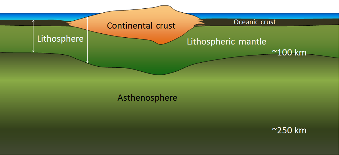
Boundaries between the plates are of three types: divergent (i.e., moving apart), convergent (i.e., moving together), and transform (moving side by side). The plates are made up of crust and the lithospheric part of the mantle (Figure 10.4.2), and even though they are moving all the time, and in different directions, there is never a significant amount of space between them. Plates are thought to move along the lithosphere-asthenosphere boundary, as the asthenosphere is the zone of partial melting. It is assumed that the relative lack of strength of the partial melting zone facilitates the sliding of the lithospheric plates.
It is possible for a single plate to be made up of both oceanic and continental crust. For example, the North American Plate includes most of North America, plus half of the northern Atlantic Ocean. Similarly, the South American Plate extends across the western part of the southern Atlantic Ocean, while the European and African plates each include part of the eastern Atlantic Ocean. The Pacific Plate is almost entirely oceanic, but it does include the part of California west of the San Andreas Fault.
Divergent Boundaries
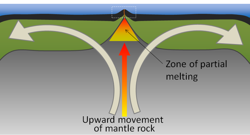
Divergent boundaries are spreading boundaries, where new oceanic crust is created from magma derived from partial melting of the mantle caused by decompression as hot mantle rock from depth is moved toward the surface (Figure 10.4.3). Most divergent boundaries are located at the oceanic ridges (although some are on land), and the crustal material created at a spreading boundary is always oceanic in character. Spreading rates vary considerably, from 2 cm/y to 6 cm/y in the Atlantic, to between 12 cm/y and 20 cm/y in the Pacific.
Some of the processes taking place in this setting include:
- Magma from the mantle pushing up to fill the voids left by divergence of the two plates.
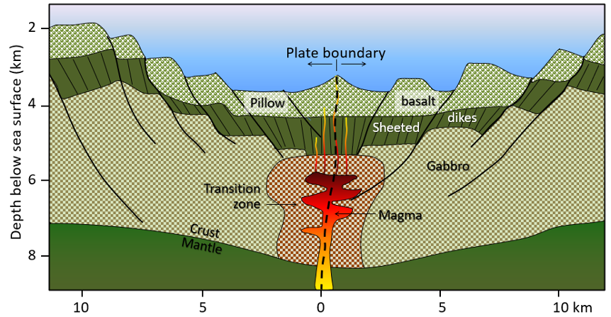
- Pillow lavas forming where magma is pushed out into seawater (Figure 10.4.4).
- Vertical sheeted dykes intruding into cracks resulting from the spreading.
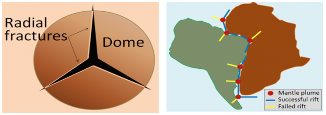
Spreading is hypothesized to start within a continental area with up-warping or doming related to an underlying mantle plume or series of mantle plumes. The buoyancy of the mantle plume material creates a dome within the crust, causing it to fracture in a radial pattern, with three arms spaced at approximately 120° (Figure 10.4.5). When a series of mantle plumes exists beneath a large continent, the resulting rifts may align and lead to the formation of a rift valley (such as the present-day Great Rift Valley in eastern Africa). It is suggested that this type of valley eventually develops into a linear sea (such as the present-day Red Sea), and finally into an ocean (such as the Atlantic). It is likely that as many as 20 mantle plumes, many of which still exist, were responsible for the initiation of the rifting of Pangea along what is now the mid-Atlantic ridge.
Convergent Boundaries
Convergent boundaries, where two plates are moving toward each other, are of three types, depending on whether oceanic or continental crust is present on either side of the boundary. The types are ocean-ocean, ocean-continent, and continent-continent.
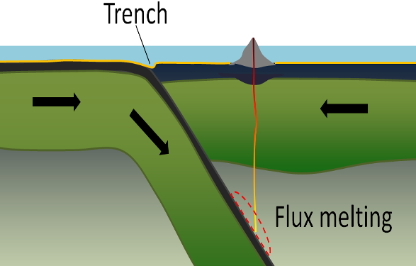
At an ocean-ocean convergent boundary, one of the plates (oceanic crust and lithospheric mantle) is pushed, or subducted, under the other. Often it is the older and colder plate that is denser and subducts beneath the younger and hotter plate. There is commonly an ocean trench along the boundary. The subducted lithosphere descends into the hot mantle at a relatively shallow angle close to the subduction zone, but at steeper angles farther down (up to about 45°). The significant volume of water within the subducting material is released as the subducting crust is heated. It is released when the oceanic crust is heated and then rises and mixes with the overlying mantle. The addition of water to the hot mantle lowers the rocks’ melting point and leads to the formation of magma (flux melting) (Figure 10.4.6). The magma, which is lighter than the surrounding mantle material, rises through the mantle and the overlying oceanic crust to the ocean floor where it creates a chain of volcanic islands known as an island arc. A mature island arc develops into a chain of relatively large islands (such as Japan or Indonesia) as more and more volcanic material is extruded and sedimentary rocks accumulate around the islands.
Earthquakes take place close to the boundary between the subducting crust and the overriding crust. The largest earthquakes occur near the surface where the subducting plate is still cold and strong.
Examples of ocean-ocean convergent zones are subduction of the Pacific Plate beneath the North America Plate south of Alaska (Aleutian Islands) and beneath the Philippine Plate west of the Philippines, subduction of the India Plate beneath the Eurasian Plate south of Indonesia, and subduction of the Atlantic Plate beneath the Caribbean Plate (see Figure 10.4.1).
At an ocean-continent convergent boundary, the oceanic plate is pushed under the continental plate in the same manner as at an ocean-ocean boundary. Sediment that has accumulated on the continental slope is thrust up into an accretionary wedge, and compression leads to thrusting within the continental plate (Figure 10.4.7). The mafic magma produced adjacent to the subduction zone rises to the base of the continental crust and leads to partial melting of the crustal rock. The resulting magma ascends through the crust, producing a mountain chain with many volcanoes.
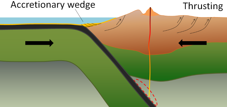
Examples of ocean-continent convergent boundaries are subduction of the Nazca Plate under South America (which has created the Andes Range) and subduction of the Juan de Fuca Plate under North America (creating the mountains Garibaldi, Baker, St. Helens, Rainier, Hood, and Shasta, collectively known as the Cascade Range).
A continent-continent collision occurs when a continent or large island that has been moved along with subducting oceanic crust collides with another continent (Figure 10.4.8). The colliding continental material will not be subducted because it is too light (i.e., because it is composed largely of light continental rocks), but the root of the oceanic plate will eventually break off and sink into the mantle. There is tremendous deformation of the pre-existing continental rocks, and creation of mountains from that rock, from any sediments that had accumulated along the shores (i.e., within geosynclines) of both continental masses, and commonly also from some ocean crust and upper mantle material.
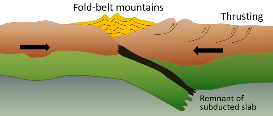
Examples of continent-continent convergent boundaries are the collision of the India Plate with the Eurasian Plate, creating the Himalaya Mountains, and the collision of the African Plate with the Eurasian Plate, creating the series of ranges extending from the Alps in Europe to the Zagros Mountains in Iran. The Rocky Mountains in B.C. and Alberta are also a result of continent-continent collisions.
Transform Boundaries
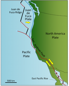
Transform boundaries exist where one plate slides past another without production or destruction of crustal material. As explained above, most transform faults connect segments of mid-ocean ridges and are thus ocean-ocean plate boundaries. Some transform faults connect continental parts of plates. An example is the San Andreas Fault, which extends from the southern end of the Juan de Fuca Ridge to the northern end of the East Pacific Rise (ridge) in the Gulf of California (Figures 10.4.9 and 10.4.10). The part of California west of the San Andreas Fault and all of Baja California are on the Pacific Plate. Transform faults do not just connect divergent boundaries. For example, the Queen Charlotte Fault connects the north end of the Juan de Fuca Ridge, starting at the north end of Vancouver Island, to the Aleutian subduction zone.
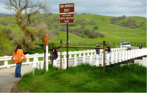
Figure 10.4.10 The San Andreas Fault at Parkfield in central California. The person with the orange shirt is standing on the Pacific Plate and the person at the far side of the bridge is on the North American Plate. The bridge is designed to accommodate motion on the fault by sliding on its foundation.
Geological Time
In 1788, after many years of geological study, James Hutton, one of the great pioneers of geology, wrote the following about the age of Earth: The result, therefore, of our present enquiry is, that we find no vestige of a beginning — no prospect of an end.[1] Of course he wasn’t exactly correct, there was a beginning and there will be an end to Earth, but what he was trying to express is that geological time is so vast that we humans, who typically live for less than a century, have no means of appreciating how much geological time there is. Hutton didn’t even try to assign an age to Earth, but we now know that it is approximately 4,570 million years old. Using the scientific notation for geological time, that is 4,570 Ma (for mega annum or “millions of years”) or 4.57 Ga (for giga annum or billions of years). More recent dates can be expressed in ka (kilo annum); for example, the last cycle of glaciation ended at approximately 11.7 ka or 11,700 years ago.
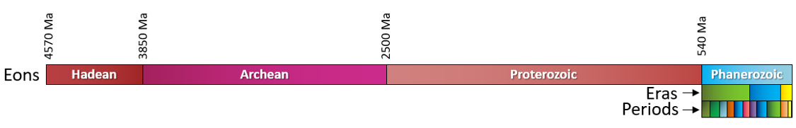
Unfortunately, knowing how to express geological time doesn’t really help us understand or appreciate its extent. A version of the geological time scale is included as Figure 1.6.1. Unlike time scales you’ll see in other places, this time scale is linear throughout its length, meaning that 50 Ma during the Cenozoic is the same thickness as 50 Ma during the Hadean. Most other time scales have earlier parts of Earth’s history compressed so that more detail can be shown for the more recent parts. That makes it difficult to appreciate the extent of geological time.
To create some context, the Phanerozoic Eon (the last 542 million years) is named for the time during which visible (phaneros) life (zoi) is present in the geological record. In fact, large organisms—those that leave fossils visible to the naked eye—have existed for a little longer than that, first appearing around 600 Ma, or a span of just over 13% of geological time. Animals have been on land for 360 million years, or 8% of geological time. Mammals have dominated since the demise of the dinosaurs around 65 Ma, or 1.5% of geological time, and the genus Homo has existed since approximately 2.8 Ma, or 0.06% (1/1,600th) of geological time.
Geologists (and geology students) need to understand geological time. That doesn’t mean memorizing the geological time scale; instead, it means getting your mind around the concept that although most geological processes are extremely slow, very large and important things can happen if such processes continue for enough time.
For example, the Atlantic Ocean between Nova Scotia and northwestern Africa has been getting wider at a rate of about 2.5 centimetres (cm) per year. Imagine yourself taking a journey at that rate—it would be impossibly and ridiculously slow. And yet, since it started to form at around 200 Ma (just 4% of geological time), the Atlantic Ocean has grown to a width of over 5,000 kilometres (km)!
A useful mechanism for understanding geological time is to scale it all down into one year. The origin of the solar system and Earth at 4.57 Ga would be represented by January 1, and the present year would be represented by the last tiny fraction of a second on New Year’s Eve. At this scale, each day of the year represents 12.5 million years; each hour represents about 500,000 years; each minute represents 8,694 years; and each second represents 145 years. Some significant events in Earth’s history, as expressed on this time scale, are summarized on Table 1.1.
|
Event |
Approximate Date |
Calendar Equivalent |
|---|---|---|
|
Formation of oceans and continents |
4.5 to 4.4 Ga |
January |
|
Evolution of the first primitive life forms |
3.8 Ga |
early March |
|
Formation of British Columbia’s oldest rocks |
2.0 Ga |
July |
|
Evolution of the first multi-celled animals |
0.6 Ga or 600 Ma |
November 15 |
|
Animals first crawled onto land |
360 Ma |
December 1 |
|
Vancouver Island reached North America and the Rocky Mountains were formed |
90 Ma |
December 25 |
|
Extinction of the non-avian dinosaurs |
65 Ma |
December 26 |
|
Beginning of the Pleistocene ice age |
2 Ma or 2000 ka |
8 p.m., December 31 |
|
Retreat of the most recent glacial ice from southern Canada |
14 ka |
11:58 p.m., December 31 |
|
Arrival of the first people in British Columbia |
10 ka |
11:59 p.m., December 31 |
|
Arrival of the first Europeans on the west coast of what is now Canada |
250 years ago |
2 seconds before midnight, December 31 |
Measuring Geological Time
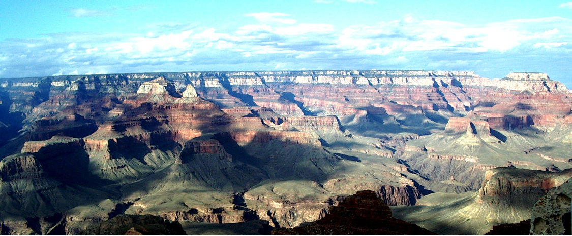
Time is the dimension that sets geology apart from most other sciences. Geological time is vast, and Earth has changed enough over that time that some of the rock types that formed in the past could not form today. Furthermore, even though most geological processes are very, very slow, the vast amount of time that has passed has allowed for the formation of extraordinary geological features, as shown in Figure 8.0.1.
We have numerous ways of measuring geological time. We can tell the relative ages of rocks (for example, whether one rock is older than another) based on their spatial relationships; we can use fossils to date sedimentary rocks because we have a detailed record of the evolution of life on Earth; and we can use a range of isotopic techniques to determine the actual ages (in millions of years) of igneous and metamorphic rocks.
But just because we can measure geological time doesn’t mean that we understand it. One of the biggest hurdles faced by geology students—and geologists as well—in mastering geology, is to really come to grips with the slow rates at which geological processes happen and the vast amount of time involved.
The Geological Time Scale
William Smith worked as a surveyor in the coal-mining and canal-building industries in southwestern England in the late 1700s and early 1800s. While doing his work, he had many opportunities to look at the Paleozoic and Mesozoic sedimentary rocks of the region, and he did so in a way that few had done before. Smith noticed the textural similarities and differences between rocks in different locations, and more importantly, he discovered that fossils could be used to correlate rocks of the same age. Smith is credited with formulating the principle of fauna succession (the concept that specific types of organisms lived during different time intervals), and he used it to great effect in his monumental project to create a geological map of England and Wales, published in 1815.
Inset into Smith’s great geological map is a small diagram showing a schematic geological cross-section extending from the Thames estuary of eastern England all the way to the west coast of Wales. Smith shows the sequence of rocks, from the Paleozoic rocks of Wales and western England, through the Mesozoic rocks of central England, to the Cenozoic rocks of the area around London (Figure 8.1.1). Although Smith did not put any dates on these—because he didn’t know them—he was aware of the principle of superposition (the idea, developed much earlier by the Danish theologian and scientist Nicholas Steno, that young sedimentary rocks form on top of older ones), and so he knew that this diagram represented a stratigraphic column. And because almost every period of the Phanerozoic is represented along that section through Wales and England, it is a primitive geological time scale.
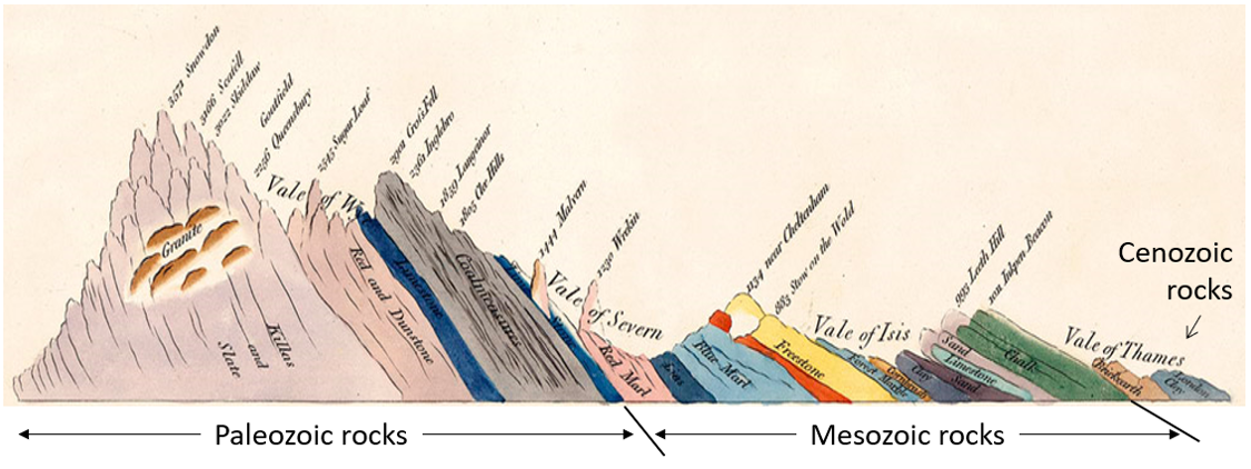
Smith’s work set the stage for the naming and ordering of the geological periods, which was initiated around 1820, first by British geologists, and later by other European geologists. Many of the periods are named for places where rocks of that age are found in Europe, such as Cambrian for Cambria (Wales), Devonian for Devon in England, Jurassic for the Jura Mountains in France and Switzerland, and Permian for the Perm region of Russia. Some are named for the type of rock that is common during that age, such as Carboniferous for the coal- and carbonate-bearing rocks of England, and Cretaceous for the chalks of England and France.
The early time scales were only relative because 19th century geologists did not know the ages of the rocks. That information was not available until the development of isotopic dating techniques early in the 20th century.
The geological time scale is currently maintained by the International Commission on Stratigraphy (ICS), which is part of the International Union of Geological Sciences. The time scale is continuously being updated as we learn more about the timing and nature of past geological events. You can view the ICS time scale[2] online. There is a downloaded copy in this unit on D2L. It would be a good idea to print a copy (in colour) to put on your wall while you are studying geology.
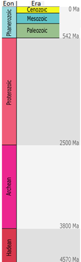
Geological time has been divided into four eons: Hadean (4570 to 4850 Ma), Archean (3850 to 2500 Ma), Proterozoic (2500 to 540 Ma), and Phanerozoic (540 Ma to present). As shown in Figure 8.1.2, the first three of these represent almost 90% of Earth’s history. The last one, the Phanerozoic (meaning “visible life”), is the time that we are most familiar with because Phanerozoic rocks are the most common on Earth, and they contain evidence of the life forms that we are familiar with to varying degrees.
The Phanerozoic eon—the past 540 Ma of Earth’s history—is divided into three eras: the Paleozoic (“early life”), the Mesozoic (“middle life”), and the Cenozoic (“new life”), and each of these is divided into a number of periods (Figure 8.1.3). Most of the organisms that we share Earth with evolved at various times during the Phanerozoic.
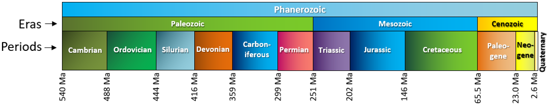
Figure 8.1.3 image description: The eras and periods that make up the Phanerozoic Eon
|
Era |
Period |
Time span |
|---|---|---|
|
Paleozoic |
Cambrian |
488 to 540 Ma |
|
Paleozoic |
Ordovician |
488 to 444 Ma |
|
Paleozoic |
Silurian |
444 to 416 Ma |
|
Paleozoic |
Devonian |
416 to 359 Ma |
|
Paleozoic |
Carboniferous |
359 to 299 Ma |
|
Paleozoic |
Permian |
299 to 251 Ma |
|
Mesozoic |
Triassic |
251 to 202 Ma |
|
Mesozoic |
Jurassic |
202 to 146 Ma |
|
Mesozoic |
Cretaceous |
146 to 65.5 Ma |
|
Cenozoic |
Paleogene |
65.5 to 23 Ma |
|
Cenozoic |
Neogene |
23 to 2.6 Ma |
|
Cenozoic |
Quaternary |
2.6 Ma to present |
The Cenozoic era, which represents the past 65.5 Ma, is divided into three periods: Paleogene, Neogene, and Quaternary, and seven epochs (Figure 8.1.4). Dinosaurs became extinct at the start of the Cenozoic, after which birds and mammals radiated to fill the available habitats. Earth was very warm during the early Eocene and has steadily cooled ever since. Glaciers first appeared on Antarctica in the Oligocene and then on Greenland in the Miocene, and covered much of North America and Europe by the Pleistocene. The most recent of the Pleistocene glaciations ended around 11,700 years ago. The current epoch is known as the Holocene. Epochs are further divided into ages (a.k.a. stages), but we won’t be going into that level of detail here.
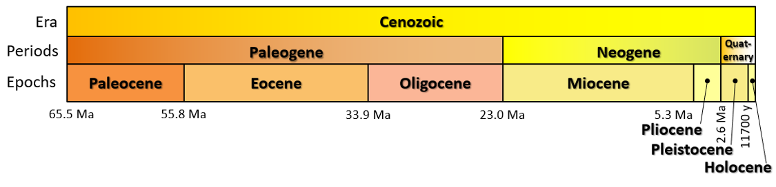
Figure 8.1.4 image description: The periods and epochs that make up the Cenozoic era
|
Period |
Epoch |
Time span |
|---|---|---|
|
Paleogene |
Paleocene |
65.5 to 55.8 Ma |
|
Paleogene |
Eocene |
55.8 to 33.9 Ma |
|
Paleogene |
Oligocene |
33.9 to 23.0 Ma |
|
Neogene |
Miocene |
23.0 to 5.3 Ma |
|
Neogene |
Pliocene |
5.3 to 2.6 Ma |
|
Quaternary |
Pleistocene |
2.6 Ma to 11,700 years ago |
|
Quaternary |
Holocene |
11,700 years ago to the present |
Most of the boundaries between the periods and epochs of the geological time scale have been fixed on the basis of significant changes in the fossil record. For example, as already noted, the boundary between the Cretaceous and the Paleogene coincides exactly with a devastating mass extinction. That’s not a coincidence. The dinosaurs and many other types of organisms went extinct at this time, and the boundary between the two periods marks the division between sedimentary rocks with Cretaceous organisms (including dinosaurs) below, and Paleogene organisms above.
Relative Dating Methods
The simplest and most intuitive way of dating geological features is to look at the relationships between them. There are a few simple rules for doing this. For example, the principle of superposition states that sedimentary layers are deposited in sequence, and, unless the entire sequence has been turned over by tectonic processes or disrupted by faulting, the layers at the bottom are older than those at the top. The principal of inclusion states that any rock fragments that are included in rock must be older than the rock in which they are included. For example, a xenolith in an igneous rock or a clast in sedimentary rock must be older than the rock that includes it (Figure 8.2.1).
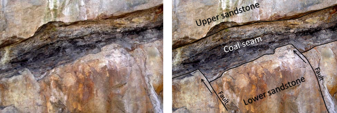
The principle of cross-cutting relationships states that any geological feature that cuts across, or disrupts another feature must be younger than the feature that is disrupted. An example of this is given in Figure 8.2.2, which shows three different sedimentary layers. The lower sandstone layer is disrupted by two faults, so we can conclude that the faults are younger than that layer. But the faults do not appear to continue into the coal seam, and they certainly do not continue into the upper sandstone. So we can infer that coal seam is younger than the faults (because it cuts them off), and of course the upper sandstone is youngest of all, because it lies on top of the coal seam.
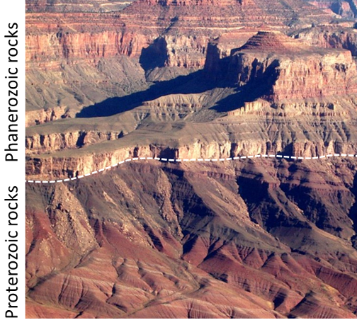
An unconformity represents an interruption in the process of deposition of sedimentary rocks. Recognizing unconformities is important for understanding time relationships in sedimentary sequences. An example of an unconformity is shown in Figure 8.2.4. The Proterozoic rocks of the Grand Canyon Group have been tilted and then eroded to a flat surface prior to deposition of the younger Paleozoic rocks. The difference in time between the youngest of the Proterozoic rocks and the oldest of the Paleozoic rocks is close to 300 million years. Tilting and erosion of the older rocks took place during this time, and if there was any deposition going on in this area, the evidence of it is now gone.
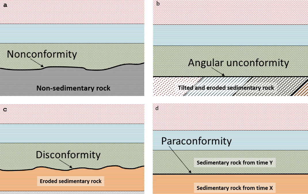
There are four types of unconformities, as summarized in Table 8.1, and illustrated in Figure 8.2.5.
Table 8.1 The characteristics of the four types of unconformities
|
Unconformity Type |
Description |
|---|---|
|
Nonconformity |
A boundary between non-sedimentary rocks (below) and sedimentary rocks (above) |
|
Angular unconformity |
A boundary between two sequences of sedimentary rocks where the underlying ones have been tilted (or folded) and eroded prior to the deposition of the younger ones (as in Figure 8.2.4) |
|
Disconformity |
A boundary between two sequences of sedimentary rocks where the underlying ones have been eroded (but not tilted) prior to the deposition of the younger ones (as in Figure 8.2.2) |
|
Paraconformity |
A time gap in a sequence of sedimentary rocks that does not show up as an angular unconformity or a disconformity |
Dating Rocks Using Fossils
Geologists get a wide range of information from fossils. They help us to understand evolution and life in general; they provide critical information for understanding depositional environments and changes in Earth’s climate; and, of course, they can be used to date rocks.
Although the recognition of fossils goes back hundreds of years, the systematic cataloguing and assignment of relative ages to different organisms from the distant past—paleontology—only dates back to the earliest part of the 19th century. The oldest undisputed fossils are from rocks dated around 3.5 Ga, and although fossils this old are tiny, typically poorly preserved and are not useful for dating rocks, they can still provide important information about conditions at the time. The oldest well-understood fossils are from rocks dating back to around 600 Ma, and the sedimentary record from that time forward is rich in fossil remains that provide a detailed record of the history and evolution of life on Earth. However, as anyone who has gone hunting for fossils knows, that does not mean that all sedimentary rocks have visible fossils, or that they are easy to find. Fossils alone cannot provide us with numerical ages of rocks, but over the past century geologists have acquired enough isotopic dates from rocks associated with fossil-bearing rocks (such as igneous dykes cutting through sedimentary layers, or volcanic layers between sedimentary layers) to be able to put specific time limits on most fossils.
A very selective history of life on Earth over the past 600 million years is provided in Figure 8.3.1. The major groups of organisms that we are familiar with evolved between the late Proterozoic and the Cambrian (approximately 600 to 520 Ma). Plants, which evolved in the oceans as green algae, came onto land during the Ordovician (approximately 450 Ma). Insects, which evolved from marine arthropods, came onto land during the Devonian (400 Ma), and amphibians (i.e., vertebrates) came onto land about 50 million years later. By the late Carboniferous, trees had evolved from earlier plants, and reptiles had evolved from amphibians. By the mid-Triassic, dinosaurs and mammals had evolved from very different branches of the reptiles; birds evolved from dinosaurs during the Jurassic. Flowering plants evolved in the late Jurassic or early Cretaceous. The earliest primates evolved from other mammals in the early Paleogene, and the genus Homo evolved during the late Neogene (roughly 2.8 Ma).
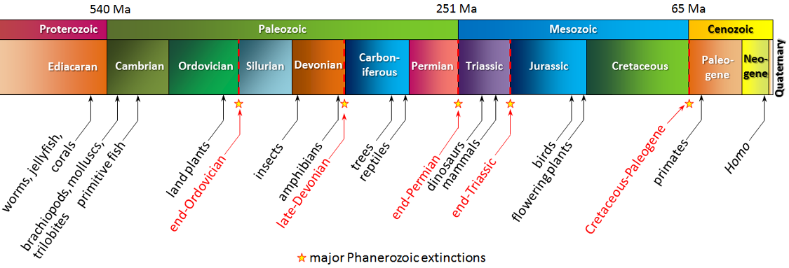
Figure 8.3.1 image description: Life on earth during the late Proterozoic and the Phanerozoic
|
Eon |
Ero |
Period |
Life on Earth |
|---|---|---|---|
|
Proterozoic |
|
Ediacaran |
Worms, jellyfish, corals |
|
Phanerozoic |
Paleozoic (540 to 251 Ma) |
Cambrian |
Brachiopods, molluscs, trilobites, primitive fish |
|
Phanerozoic |
Paleozoic (540 to 251 Ma) |
Ordovician |
Land plants, the period ends with a major extinction |
|
Phanerozoic |
Paleozoic (540 to 251 Ma) |
Silurian |
|
|
Phanerozoic |
Paleozoic (540 to 251 Ma) |
Devonian |
Insects, amphibians, the period ends with a major extinction |
|
Phanerozoic |
Paleozoic (540 to 251 Ma) |
Carboniferous |
Trees, reptiles |
|
Phanerozoic |
Paleozoic (540 to 251 Ma) |
Permian |
The period ends with a major extinction |
|
Phanerozoic |
Mesozoic (251 to 65 Ma) |
Triassic |
Dinosaurs, mammals, the period ends with a major extinction |
|
Phanerozoic |
Mesozoic (251 to 65 Ma) |
Jurrassic |
Birds, flowering plants |
|
Phanerozoic |
Mesozoic (251 to 65 Ma) |
Cretaceous |
The period ends with a major extinction |
|
Phanerozoic |
Cenozoic, (65 Ma to present) |
Paleogene |
Primates |
|
Phanerozoic |
Cenozoic, (65 Ma to present) |
Neogene |
Homo |
|
Phanerozoic |
Cenozoic, (65 Ma to present) |
Quaternary |
If we understand the sequence of evolution on Earth, we can apply knowledge to determining the relative ages of rocks. This is William Smith’s principle of faunal succession, although of course it doesn’t just apply to “fauna” (animals); it can also apply to fossils of plants and those of simple organisms.
The Phanerozoic has seen five major extinctions, as indicated in Figure 8.3.1. The most significant of these was at the end of the Permian, which saw the extinction of over 80% of all species and over 90% of all marine species. Most well-known types of organisms were decimated by this event, but only a few became completely extinct, including trilobites. The second most significant extinction was at the Cretaceous-Paleogene boundary (K-Pg, a.k.a. the K-T extinction). At that time, about 75% of marine species disappeared. Again, a few well-known types of organisms disappeared altogether, including the dinosaurs (but not birds) and the pterosaurs. Many other types were badly decimated by that event but survived, and then flourished in the Paleogene. The K-Pg extinction is thought to have been caused by the impact of a large extraterrestrial body (10 to 15 kilometres across), but it is generally agreed that the other four Phanerozoic extinctions had other causes, although their exact nature is not clearly understood.
It is no coincidence that the major extinctions all coincide with boundaries of geological periods and even eras. Geologists have placed most of the divisions of the geological time scale at points in the fossil record where there are major changes in the type of organisms observed, and most of these correspond with minor or major extinctions.
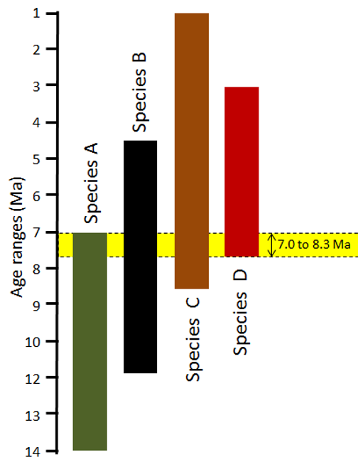
If we can identify a fossil to the species level, or at least to the genus level, and we know the time period when the organism lived, we can assign a range of time to the rock. That range might be several million years because some organisms survived for a very long time. If the rock we are studying has several types of fossils in it, and we can assign time ranges to several of them, we might be able to narrow the time range for the age of the rock considerably. An example of this is given in Figure 8.3.2.
Some organisms survived for a very long time, and are not particularly useful for dating rocks. Sharks, for example, have been around for over 400 million years, and the great white shark has survived for 16 million years, so far. Organisms that lived for relatively short time periods are particularly useful for dating rocks, especially if they were distributed over a wide geographic area and so can be used to compare rocks from different regions. These are known as index fossils. There is no specific limit on how short the time span has to be to qualify as an index fossil. Some lived for millions of years, and others for much less than a million years.
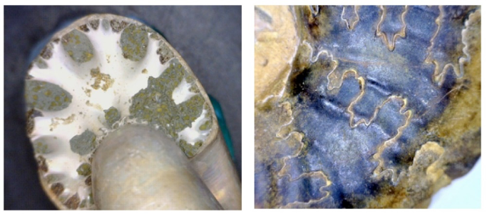
Some well-studied groups of organisms qualify as biozone fossils because, although the genera and families lived over a long time, each species lived for a relatively short time and can be easily distinguished from others on the basis of specific features. For example, ammonites have a distinctive feature known as the suture line—where the internal shell layers that separate the individual chambers (septae) meet the outer shell wall, as shown in Figure 8.3.3. These suture lines are sufficiently variable to identify species that can be used to estimate the relative or absolute ages of the rocks in which they are found.
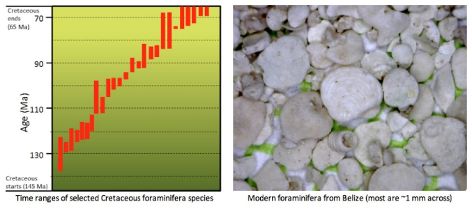
Foraminifera (small, carbonate-shelled marine organisms that originated during the Triassic and are still around today) are also useful biozone fossils. As shown in Figure 8.3.4, numerous different foraminifera lived during the Cretaceous. Some lasted for over 10 million years, but others for less than 1 million years. If the foraminifera in a rock can be identified to the species level, we can get a good idea of its age.
Isotopic Dating Methods
Originally fossils only provided us with relative ages because, although early paleontologists understood biological succession, they did not know the absolute ages of the different organisms. It was only in the early part of the 20th century, when isotopic dating methods were first applied, that it became possible to discover the absolute ages of the rocks containing fossils. In most cases, we cannot use isotopic techniques to directly date fossils or the sedimentary rocks they are found in, but we can constrain their ages by dating igneous rocks that cut across sedimentary rocks, or volcanic layers that lie within sedimentary layers.
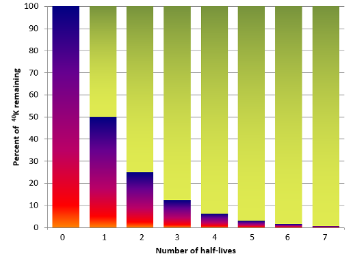
Figure 8.4.1 image description: Decay of 40K over time
|
Number of half-lives |
Percent of 40K remaining |
Percent of 40Ar |
|---|---|---|
|
0 |
100 |
0 |
|
1 |
50 |
50 |
|
2 |
25 |
75 |
|
3 |
12.5 |
87.5 |
|
4 |
6.25 |
93.75 |
|
5 |
3.125 |
96.875 |
|
6 |
1.5625 |
98.4375 |
|
7 |
0.78125 |
99.21875 |
Isotopic dating of rocks, or the minerals in them, is based on the fact that we know the decay rates of certain unstable isotopes of elements and that these rates have been constant over geological time. It is also based on the premise that when the atoms of an element decay within a mineral or a rock, they stay there and don’t escape to the surrounding rock, water, or air. One of the isotope pairs widely used in geology is the decay of 40K to 40Ar (potassium-40 to argon-40). 40K is a radioactive isotope of potassium that is present in very small amounts in all minerals that have potassium in them. It has a half-life of 1.3 billion years, meaning that over a period of 1.3 Ga one-half of the 40K atoms in a mineral or rock will decay to 40Ar, and over the next 1.3 Ga one-half of the remaining atoms will decay, and so on (Figure 8.4.1).
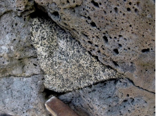
In order to use the K-Ar dating technique, we need to have an igneous or metamorphic rock that includes a potassium-bearing mineral. One good example is granite, which normally has some potassium feldspar (Figure 8.4.2). Feldspar does not have any argon in it when it forms. Over time, the 40K in the feldspar decays to 40Ar. Argon is a gas and the atoms of 40Ar remain embedded within the crystal, unless the rock is subjected to high temperatures after it forms. The sample must be analyzed using a very sensitive mass-spectrometer, which can detect the differences between the masses of atoms, and can therefore distinguish between 40K and the much more abundant 39K. Biotite and hornblende are also commonly used for K-Ar dating.
Why can’t we use isotopic dating techniques to accurately date sedimentary rocks?
K-Ar is just one of many isotope-pairs that are useful for dating geological materials. Some of the other important pairs are listed in Table 8.2, along with the age ranges that they apply to and some comments on their applications. When radiometric techniques are applied to metamorphic rocks, the results normally tell us the date of metamorphism, not the date when the parent rock formed.
Table 8.2 A few of the isotope systems that are widely used for dating geological materials
|
Isotope System |
Half-Life |
Useful Range |
Comments |
|---|---|---|---|
|
Potassium-argon |
1.3 Ga |
10 Ka to 4.57 Ga |
Widely applicable because most rocks have some potassium |
|
Uranium-lead |
4.5 Ga |
1 Ma to 4.57 Ga |
The rock must have uranium-bearing minerals, but most have enough. |
|
Rubidium-strontium |
47 Ga |
10 Ma to 4.57 Ga |
Less precision than other methods at old dates |
|
Carbon-nitrogen (a.k.a. radiocarbon dating) |
5,730 years |
100 to 60,000 years |
Sample must contain wood, bone, or carbonate minerals; can be applied to young sediments |
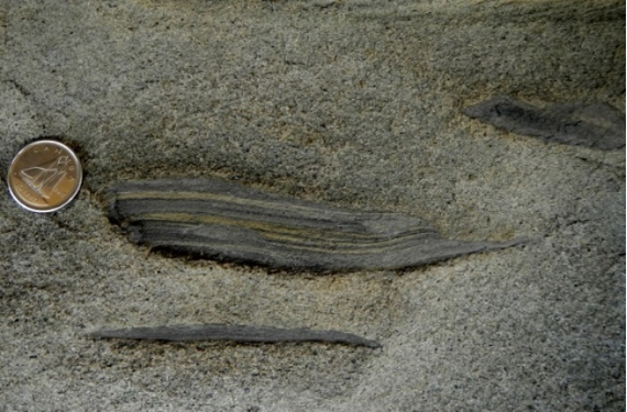
Radiocarbon dating (using 14C) can be applied to many geological materials, including sediments and sedimentary rocks, but the materials in question must be younger than 60 ka. Fragments of wood incorporated into young sediments are good candidates for carbon dating, and this technique has been used widely in studies involving late Pleistocene glaciers and glacial sediments.
Over the past decade there has been increasing use of U-Pb dating to study sedimentary rocks, not necessarily to find out the age of the rock, but to discover something about its history and origins. All clastic sedimentary rocks contain some tiny clasts of the silicate mineral zircon (ZrSiO4), derived from the weathering of the sediment parent rocks. Zircon always has some uranium in it (but no lead) so it is a good candidate for U-Pb dating, and it isn’t too difficult to separate the grains of zircon from the other grains in a sandstone. The procedure is to isolate a few hundred tiny zircons from a rock sample, and then carry out U-Pb dating on each one of them.
Other Dating Methods
There are numerous other techniques for dating geological materials, but we will examine just two of them here: tree-ring dating (i.e., dendrochronology) and dating based on the record of reversals of Earth’s magnetic field.
Dendrochronology can be applied to dating very young geological materials based on reference records of tree-ring growth going back many millennia. The longest such records can take us back to 25 ka, to the height of the last glaciation. One of the advantages of dendrochronology is that, providing reliable reference records are available, the technique can be used to date events to the nearest year.
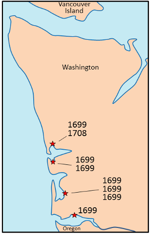
Dendrochronology has been used to date the last major subduction-zone earthquake on the coast of B.C., Washington, and Oregon. When large earthquakes strike in this setting, there is a tendency for some coastal areas to subside by one or two metres. Seawater then rushes in, flooding coastal flats and killing trees and other vegetation within a few months. There are at least four locations along the coast of Washington that have such dead trees (and probably many more in other areas). Wood samples from these trees have been studied and the ring patterns have been compared with patterns from old living trees in the region (Figure 8.5.1).
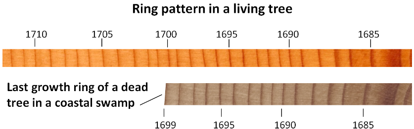
At all of the locations studied, the trees were found to have died either in the year 1699, or very shortly thereafter (Figure 8.5.2). On the basis of these results, it was concluded that a major earthquake took place in this region sometime between the end of growing season in 1699 and the beginning of the growing season in 1700. Evidence from a major tsunami that struck Japan on January 27, 1700, narrowed the timing of the earthquake to sometime in the evening of January 26, 1700.
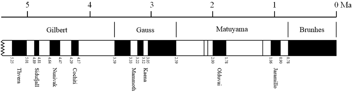
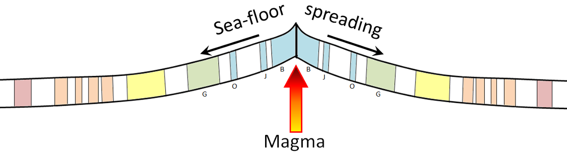
Changes in Earth’s magnetic field can also be used to date events in geologic history. The magnetic field makes compasses point toward the North Pole, but, as we’ll see in Chapter 10, this hasn’t always been the case. At various times in the past, Earth’s magnetic field has reversed itself completely, and during those times a compass would have pointed to the South Pole. By studying magnetism in volcanic rocks that have been dated isotopically, geologists have been able to delineate the chronology of magnetic field reversals going back to 250 Ma. About 5 million years of this record is shown in Figure 8.5.3, where the black bands represent periods of normal magnetism (“normal” meaning similar to the current magnetic field) and the white bands represent periods of reversed magnetism. These periods of consistent magnetic polarity are given names to make them easier to reference. The current normal magnetic field, known as Brunhes, has lasted for the past 780,000 years. Prior to that there was a short-reversed period and then a short normal period known as Jaramillo.
Oceanic crust becomes magnetized by the magnetic field that exists as the crust forms from magma. As it cools, tiny crystals of magnetite that form within the magma become aligned with the existing magnetic field and then remain that way after all of the rock has hardened, as shown in Figure 8.5.4. Crust that is forming today is being magnetized in a “normal” sense, but crust that formed 780,000 to 900,000 years ago, in the interval between the Brunhes and Jaramillo normal periods, was magnetized in the “reversed” sense.
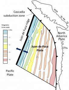
Magnetic Chronology can be used as a dating technique because we can measure the magnetic field of rocks using a magnetometer in a lab, or of entire regions by towing a magnetometer behind a ship or an airplane. For example, the Juan de Fuca Plate, which lies off of the west coast of B.C., Washington, and Oregon, is being and has been formed along the Juan de Fuca spreading ridge (Figure 8.5.5). The parts of the plate that are still close to the ridge have normal magnetism, while parts that are farther away (and formed much earlier) have either normal or reversed magnetism, depending on when the rock formed. By carefully matching the sea-floor magnetic stripes with the known magnetic chronology, we can determine the age at any point on the plate. We can see, for example, that the oldest part of the Juan de Fuca Plate that has not subducted (off the coast of Oregon) is just over 8 million years old, while the part that is subducting underneath Vancouver Island is between 0 and about 6 million years old.
Attributions:
Excerpts from: Physical Geology – 2nd Edition by Steven Earle is used under a Creative Commons Attribution CC BY 4.0 International Licence. Download for free from the B.C. Open Collection.
Modified from: Physical Geology – 2nd Edition by Steven Earle is used under a Creative Commons Attribution 4.0 International Licence. Download for free from the B.C. Open Collection.
Figure 1.1.2 by Steven Earle, CC BY 4.0
Figure 1.4.2 by Steven Earle, CC BY 4.0
Figure 3.1.1 by Steven Earle, CC BY 4.0
Figure 3.1.2 by Steven Earle, CC BY 4.0
Figure 3.1.3 by Steven Earle, CC BY 4.0
Figure 3.1.4 by Steven Earle, CC BY 4.0
Figure 1.5.1 by Steven Earle, CC BY 4.0
Figure 1.5.2 Oceanic Spreading by Surachit. Public domain.
Figure 10.1.2 “Snider-Pellegrini Wegener fossil map” by Osvaldocangaspadilla. Public domain.
Figure 10.4.1 “Plates tect2 en” by the USGS. Adapted by Steven Earle. Public domain.
Figure 10.3.8 by Steven Earle, CC BY 4.0
Figure 10.4.2 by Steven Earle, CC BY 4.0
Figure 10.4.3 by Steven Earle, CC BY 4.0
Figure 10.4.5 by Steven Earle, CC BY 4.0
Figure 10.4.6 by Steven Earle, CC BY 4.0
Figure 10.4.7 by Steven Earle, CC BY 4.0
Figure 10.4.8 by Steven Earle, CC BY 4.0
Figure 10.4.9 by Steven Earle, CC BY 4.0
Figure 10.4.10 by Steven Earle, CC BY 4.0
Figure 10.4.11 by Steven Earle, CC BY 4.0
Figure 10.4.12 by Steven Earle, CC BY 4.0
Figure 10.4.13 by Steven Earle, CC BY 4.0
Figure 10.4.14 by Steven Earle, CC BY 4.0
Figure 10.4.4 by Steven Earle, CC BY 4.0 Based on Keary and Vine, 1996, Global Tectonics (2ed), Blackwell Science Ltd., Oxford.
Figure 1.6.1 by Steven Earle, CC BY 4.0
Figure 8.0.1 by Steven Earle, CC BY 4.0
Figure 8.1.1 “Sketch of the succession of strata and their relative altitudes” by William Smith. Adapted by Steven Earle. Public domain.
Figures 8.1.2 by Steven Earle, CC BY 4.0
Figure 8.1.3 by Steven Earle, CC BY 4.0
Figure 8.1.4 by Steven Earle, CC BY 4.0
Figure 8.2.1ab by Steven Earle, CC BY 4.0
Figure 8.2.2 by Steven Earle, CC BY 4.0
Figure 8.2.3 by Steven Earle, CC BY 4.0
Figure 8.2.4 by Steven Earle, CC BY 4.0
Figure 8.2.5 by Steven Earle, CC BY 4.0
Figure 8.3.1 by Steven Earle, CC BY 4.0
Figure 8.3.2 by Steven Earle, CC BY 4.0
Figure 8.3.3 by Steven Earle, CC BY 4.0
Figure 8.3.4 by Steven Earle, CC BY 4.0
Figure 8.3.4 (left) by Steven Earle, CC BY 4.0. Based on data in R. Scott, 2014, “A Cretaceous chronostratigraphic database: construction and applications,” Carnets de Géologie, Vol. 14.
Figure 8.3.5 by Steven Earle, CC BY 4.0. Based on data at obtained from Lower Turonian Euramerican Inoceramidae: A morphologic, taxonomic, and biostratigraphic overview.
Figure 8.4.1 by Steven Earle, CC BY 4.0
Figure 8.4.2 by Steven Earle, CC BY 4.0
Figure 8.4.3 by Steven Earle, CC BY 4.0
Figure 8.4.4 by Steven Earle, CC BY 4.0
Figure 8.4.5 by Steven Earle, CC BY 4.0 From J. Clague, 1976, Quadra Sand and its relation to late Wisconsin glaciation of southeast British Columbia, Can. J. Earth Sciences, V. 13, p. 803-815.
Figure 8.4.6 “Zircon microscope” © Chd. CC BY-SA.
Figure 8.4.6b by Steven Earle, CC BY 4.0 From data in Huang, C, 2018, Refining the chronostratigraphy of the lower Nanaimo Group, Vancouver Island, Canada, using Detrital Zircon Geochronology, MSc thesis, Department of Earth Science, Simon Fraser University, 74 p.
Figure 8.5.1 by Steven Earle, CC BY 4.0
Figure 8.5.4 by Steven Earle, CC BY 4.0
Figure 8.5.5 by Steven Earle, CC BY 4.0
Figure 8.5.2 by Steven Earle, CC BY 4.0 From data in Yamaguchi, D.K., B.F. Atwater, D.E. Bunker, B.E. Benson, and M.S. Reid. 1997. Tree-ring dating the 1700 Cascadia earthquake. Nature, Vol. 389, pp. 922 – 923, 30 October 1997.
Figure 8.5.3 “Geomagnetic polarity late Cenozoic” by the USGS. Adapted by Steven Earle. Public domain.
References:
1 Hutton, J, 1788. Theory of the Earth; or an investigation of the laws observable in the composition, dissolution, and restoration of land upon the Globe. Transactions of the Royal Society of Edinburgh
2 Cohen, K.M., Harper, D.A.T., Gibbard, P.L. 2023. ICS International Chronostratigraphic Chart 2023/09. International Commission on Stratigraphy,IUGS. www.stratigraphy.org (visited: 2023/12/02)
