41 Using Excel to Create the Long-Term Forecast

Creating a budget in Excel can be very simple or extremely complex, depending on the size and complexity of the business and the number of formulas and dependencies that are written into the Excel workbook.

Creating the forecast in Excel follows the same steps and flow we just explored in this chapter but with the power of a software program to do the math for you. We begin with the sales forecast, which uses several key formulas in Excel.

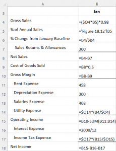
1. First, sales are projected to be 18% higher than the prior year. Thus, a total projection for the year is calculated using a simple link and multiplication function tied to last year’s total sales. In Figure 4.19, you can see the formula in cell O4 is “=’Figure 18.12′!N4*1.18”. This formula simply does the math to increase the prior year’s sales by 18%.
2. Next, the sales are distributed by month. In Figure 4.19, we see in cell B5 that the forecasted income statement sheet is linked to the percent of annual sales from the Prior Year Income Statement (Figure .12) sheet. Then, in cell B4, January sales are estimated with a formula that multiplies the total forecasted sales in O4 by the percent of annual sales for January of the prior year. Notice that the formula then multiplies that product by 0.98. This is because Clear Lake discontinued a product line in the last quarter of the prior year, and management feels that this will reduce sales in the first quarter of the new year by roughly 2%.

1. As Clear Lake continues to fill out its forecasted income statement, the next formula we see is a simple sum formula to calculate net sales in B8 (see Figure 4.20). It’s a simple formula that subtracts sales returns and allowances in B7 from gross sales in B4. Similar formulas are also found in B10 for gross margin and B18 for net income.
2. In cell B9, we see a multiplication formula that multiplies sales from B4 by 0.5, or 50%. This is because management feels that cost of goods sold will remain the same as last year, in most quarters at least, and last year’s percentage was 50%.
3. Rent, depreciation, and salaries are all simply typed in, as they are fixed expenses that remain the same as last year.
4. The utilities calculation, found in cell B14, is somewhat similar to the sales calculation. The total utilities expense from O14 is multiplied by the current month’s sales in B4 divided by the total annual sales in O4. This spreads out the utility cost by month based on the percentage of annual sales.

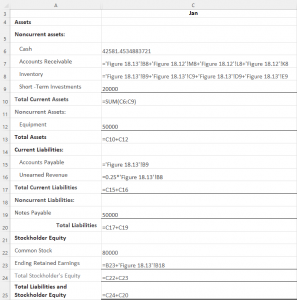
Total current assets in C10 is calculated with a SUM formula that adds together the values in all the selected cells. Amounts such as short-term investments and common stock that are not anticipated to change are simply typed as a number in the cell. Much like in the income statement, subtotals are found in C13 for total assets, C17 for current liabilities, C24 for total equity, and C25 for total liabilities and equity. Retained earnings in C23 pulls the ending retained earnings balance from the end of last year (hidden in column B) and adds the net income for January in the forecasted income statement to get the current month’s ending balance.

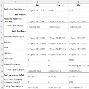
Much like the balance sheet, the cash forecast also relies heavily on data from the forecasted income statement as well as the forecasted balance sheet. To begin the year, in Figure 4.22, we see that the formula in B4 pulls the cash balance from the forecasted balance sheet. In B6, the formula pulls the sales for the three months prior from the previous year’s income statement. This is because it’s assumed that cash is collected from customers 90 days after the sale. The same approach is used for accounts payable, rent, salaries, and utilities. The formulas pull the expenses from a prior month depending on the assumed timing for payment. Utilities, for example, are assumed to be paid within 30 days, so the cash outflow in February is assumed to be the utilities expense for January from the forecasted income statement. Note that interest payments are assumed to be zero in January and February, but in March, the formula in D14 sums the interest expenses on the forecasted income statement for January, February, and March. This is because interest is paid quarterly.

Finally, note the formula in C4. The beginning cash balance for a given month is the same as the ending cash balance from the prior month; thus, the figure in B18 is linked to C4 to start the new month.

Once we get a draft of the forecasts outlined, then the tinkering starts. Additional information can be used to adjust the formulas, as we saw with the 2% reduction in January sales for the forecasted income statement. Because we have linked most (though not all) of our expenses, subtotals, and statements together using formulas, management can also use the forecast workbook to perform scenario and sensitivity analyses, essentially asking “what if?” and looking at the results. When completed, however, before finalizing the forecast, it’s important that the financial statements are in balance (particularly the balance sheet, just as the name implies).

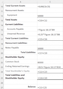
Notice that throughout, we used formulas to calculate subtotals to ensure they are correct and change as needed. We also linked figures, such as the ending and beginning cash balances, to ensure they are in balance. Perhaps the easiest but most important thing to do is to ensure that the balance sheet balances. We can do this with a simple formula that compares total assets to total liabilities and equity. We can see in Figure 4.23 that subtracting one from the other in cell C27 should result in $0. If there is a difference, the formula will highlight it, forcing us to investigate and correct the sheet so that it balances.