57 Approaches to Calculating the Cost of Capital

The Capital Asset Pricing Model

The capital asset pricing model helps investors assess the required rate of return on a given asset by measuring sensitivity to risk.

Learning Objectives

Calculate sensitivity to risk on a theoretical asset using the CAPM equation.

Key Takeaways

Key Points

  • Investors use various tools to determine the overall expected return and relative risk of a security in the broader financial markets.
  • One such tool is the capital asset pricing model (CAPM), which essentially distills the required rate of return applied to the risks (both of which are relative to the risk-free rate).
  • By utilizing the variables involved in a CAPM calculation, an investor can also determine the risk to return ratio alongside the security market line (a graphical representation of the asset’s risk and return).
  • By utilizing the CAPM equation, investors can determine when an asset is undervalued, and balance a portfolio for the best prospective return on the lowest possible risk.

Key Terms

  • capital asset pricing model: An equation that assesses the required rate of return on a given investment based upon its risk relative to a theoretical risk-free asset.

When considering assets for the diversification of an investment portfolio, investors and financiers use a variety of tools to project the required rate of return and risk of a given investment. All this really means is that investors are on the look out for ways to minimize risk, maximize returns, and invest intelligently in assets that are well-priced. The key assumption here is that the market will self-correct to adjust each investment option’s expected return to the relative risk of investing.

The Capital Asset Pricing Model

When measuring the ratio between risk and return on a given investment, the capital asset pricing model (CAPM) can be a useful tool. This model focuses on measuring a given asset’s sensitivity to systematic risk (also referred to as market risk) in relation to the expected return compared to that of a theoretical risk-free asset.

How CAPM Works

This sounds complicated, but it’s simpler than it seems. All this really means is that the CAPM tries to measure the risk the market will offer the asset compared to the risk-free rate, and make sure the expected return will offset that risk. To understand this concept, there are a few variables that are useful to identify up front:

  • E(Ri) is an expected return on security
  • E(RM) is an expected return on market portfolio M
  • β is a non-diversifiable or systematic risk
  • RM is a market rate of return
  • Rf is a risk-free rate

There are quite a few ways to rearrange the relationship between these variables to derive meaningful information. Like all equations, depending on what you know you can solve for what you don’t know as well. For a basic CAPM calculations, you would want to solve for the expected return on a security, which looks like this:


E(Ri)=Rf+βi(E(Rm)Rf){\displaystyle \text{E}(\text{R}_{\text{i}})=\text{R}_{\text{f}}+\beta _{\text{i}}(\text{E}(\text{R}_{\text{m}})-\text{R}_{\text{f}})\,}

Security Market Line

Through rearranging these variables, you can also take a look at the concept of the security market line (SML), which underlines a security’s relationship with systematic risk and respected return in a graphical format. This is written as:
 

SML:E(Ri)=Rf+βi[E(RM)Rf]{\displaystyle \mathrm {\text{SML}}:\text{E}(\text{R}_{\text{i}})=\text{R}_{\text{f}}+\beta _{\text{i}}[\text{E}(\text{R}_{\text{M}})-\text{R}_{\text{f}}]\,}

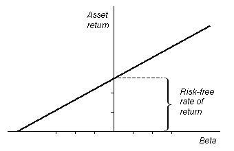
The security market line is illustrated in this graph, where an assets expected return can be visualized.
Security Market Line: The security market line is illustrated in this graph, where an assets expected return can be visualized.

Risk and Return

A final application of the CAPM variables in relation to one another is in deriving a ratio that illustrates the relationship between risk and return. On the left side of the equation below, you have an assessment of the overall risk relative to a risk-free asset. On the right side, you have the overall return (similarly relative to a risk-free asset). This can be written as follows:


E(Ri)Rfβi=E(Rm)Rf{\displaystyle {\frac {\text{E}(\text{R}_{\text{i}})-\text{R}_{\text{f}}}{\beta _{\text{i}}}}=\text{E}(\text{R}_{\text{m}})-\text{R}_{\text{f}}}

Investors can utilize the CAPM equation and its various implications to assess a variety of market investment opportunities to diversify a portfolio and identify undervalued assets.

The SML Approach

The SML is the graphical representation of CAPM used to determine if an asset is priced to offer a reasonable expected return for the risk.

Learning Objectives

Analyze assets using the Security Market Line Approach.

Key Takeaways

Key Points

  • The SML graphs the relationship between risk β ( beta ) and expected return.
  • All correctly priced assets lie on the SML.
  • If a security is priced above the SML, it is undervalued. If it is priced below the SML, it is overvalued.

Key Terms

  • slope: The ratio of the vertical and horizontal distances between two points on a line; zero if the line is horizontal, undefined if it is vertical.

The SML Approach

The Security Market Line (SML) is the graphical representation of the capital asset pricing model (CAPM), with the x-axis representing the risk (beta), and the y-axis representing the expected return. It graphs the relationship between beta (β) and expected return, i.e. it shows expected return as a function of β. The y-intercept of the SML is equal to the risk-free interest rate, while the slope is equal to the market risk premium (the market’s rate of return minus the risk-free rate). The slope also represents the risk-return tradeoff at a given time. The SML is applicable to any asset.


SML Equation: The SML is the graphical representation of CAPM, and thus is found using the same equation.

Applications of the SML

Individual assets that are correctly priced are plotted on the SML. In the ideal world of CAPM, all assets are correctly priced and thus lie on the SML. In real market scenarios, we are able to use the SML graph to determine if an asset being considered for a portfolio offers a reasonable expected return for the risk. If an asset is priced at a point above the SML, it is undervalued, since for a given amount of risk, it yields a higher return. Conversely, an asset priced below the SML is overvalued, since for a given amount of risk, it yields a lower return.

CAPM-SML: The Security Market Line for the Dow Jones Industrial Average over a 3 year period, with the x-axis representing beta and the y-axis representing expected return.


Another way to think about real market applications of the SML would be in terms of buying and selling securities. If an asset is priced above the SML, and thus undervalued, it should be bought. If an asset is priced below the SML, and thus overvalued, it should be sold.

Discounted Cash Flow Approach

A discounted cash flow analysis is a highly useful tool for calculating the net present value of a given product, process, asset, or organization.

Learning Objectives

Translate future projected cash flows into present day dollars, incorporating risk and the time value of money

Key Takeaways

Key Points

  • A discounted cash flow analysis is a highly useful tool for determining the net present value (NPV) of a given organization, process, product, or asset.
  • An NPV takes into account risk, forecasts for cash flows, and the time value of money to determine what future capital returns are worth in present-day dollars.
  • When calculating discounted cash flows over a given time period, investors and strategists must estimate the required rate of return based on assumed risk and the opportunity cost of risk-free investments (i.e. risk-free rate).
  • The most important thing for strategists and investors to remember about a discounted cash flow analysis is uncertainty, as these are future cash flows that may (or may not) occur.

Key Terms

  • nominal value: Prior to adjustment (in this context, prior to time value of money adjustments).
  • discount rate: The interest rate used to discount future cash flows into present values.

The discounted cash flow approach is a valuation method investors and organizations can use to assess the net present value (NPV) of an asset, process, product, or the overall organization. NPV analyses using the discounted cash flow approach are widely used across various industries to decide which projects to invest in. They are also used as valuation devices for investors when looking at company performance, using past performance to project future performance.

The Discounted Cash Flow Formula

The discounted cash flow formula focuses on determining the relative time value of money of each projected cash flow (i.e. monthly, quarterly, annually, etc.), bringing each forecast of future value into present value terms. Just as in an NPV analysis, the ultimate end product will be the value of future profits (or losses) in today’s terms. It’s calculated as follows:


DCF=CF1(1+r)1+CF2(1+r)2++CFn(1+r)n{\displaystyle \text{DCF}={\frac {\text{CF}_{1}}{(1+\text{r})^{1}}}+{\frac {\text{CF}_{2}}{(1+\text{r})^{2}}}+\dotsb +{\frac {\text{CF}_{\text{n}}}{(1+\text{r})^{\text{n}}}}}

In situations of multiple cash flows over multiple periods of time, it is necessary to create a summation that can incorporate variance in both variables:


DPV=t=0NFVt(1+r)t{\displaystyle \text{DPV}=\sum _{\text{t}=0}^{\text{N}}{\frac {\text{FV}_{\text{t}}}{(1+\text{r})^{\text{t}}}}}

Sometimes cash flows are considered continuous. In such scenarios, the appropriate adjustment to the equation is:


DPV=0TFV(t)eλtdt,{\displaystyle \text{DPV}=\int _{0}^{\text{T}}\text{FV}(\text{t})\,\text{e}^{-\lambda \text{t}}\text{dt}\,,} 

Inputs

When considering these formulas, you’ll need to understand your inputs. The inputs for a discounted cash flow analysis are:

  • DPV – The discounted present value of the future cash flow (FV), or FV adjusted to compensate for the units of time in the future it will be received.
  • FV – The nominal value of a cash flow amount in a future period (i.e. the amount of the cash flow prior to taking time value of money into account).
  • r – The interest rate or discount rate, which reflects two important pieces of information: the opportunity cost of foregoing other investments as well as the intrinsic risk of not receiving the projected cash flow.
  • n – The time (in a given unit of time) before the future cash flow occurs. This is usually done annually, but can be done monthly or quarterly. Keep in mind that r must be adjusted according to the time period!

Strategic Use

Like any projection, the most important thing to keep in mind as either investor or strategist is uncertainty. The primary purpose of a future cash flow analysis is to balance expectations to consider existing and future resources to make the optimal decision (from a profit perspective). As a result, determining ‘r’ (required rate of return due to opportunity cost and risk) is absolutely critical to the success of these calculations.

This is a good example of a what a discounted cash flow analysis would look like on paper, particularly as a prospective investor. There's actually quite a bit more information here than you may strictly need to understand the calculation, but it's a great way to see how each piece of information fits together.
A Discounted Cash Flow Example: This is a good example of a what a discounted cash flow analysis would look like on paper, particularly as a prospective investor. There’s actually quite a bit more information here than you may strictly need to understand the calculation, but it’s a great way to see how each piece of information fits together.

The “Bond Yield Plus Risk Premium” Approach

We can estimate the value of a company’s equity by adding its risk premium to the yield to maturity on the company’s long-term debt.

Learning Objectives

Describe the process for the bond yield plus risk premium approach

Key Takeaways

Key Points

  • The BYPRP approach applies to a company’s publicly traded equity.
  • The yield to maturity is the discount rate at which the sum of all future cash flows from a bond are equal to its price.
  • The equity risk premium is the return that stocks are expected to receive in excess of the risk-free interest rate.
  • The BYPRP approach does not produce as accurate an estimate as the capital asset pricing model or discounted cash flow analysis.


Key Terms

  • dividend yield: A company’s total annual dividend payment per share, divided by its price per share.
  • coupon payment: A periodic interest payment that the bondholder receives during the time between when the bond is issued and when it matures.
  • principal payment: The payment made upon maturity of a bond


Bond Yield Plus Risk Premium Approach

The bond yield plus risk premium (BYPRP) approach is another method we can use to determine the value of an asset, specifically, a company’s publicly traded equity. BYPRP allows us to estimate the required return on an equity by adding the equity’s risk premium to the yield to maturity on company’s long-term debt.


Bond Yield Plus Risk Premium Equation: States that the required return on an equity equals the yield of the company's long-term debt plus the equity's risk premium.
Bond Yield Plus Risk Premium Equation: States that the required return on an equity equals the yield of the company’s long-term debt plus the equity’s risk premium.


Bond Yield vs. Risk Premium

Simply put, the yield on a bond is the rate of return received from the investment. In the BYPRP approach, we use a bond’s yield to maturity, which is the discount rate at which the sum of all future cash flows from the bond (coupon payments and principal payments) are equal to the price of the bond. This is also referred to as the internal rate of return (IRR).
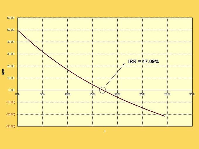
Yield To Maturity Graph: A hypothetical graph showing yield to maturities (or internal rates of return) for corresponding present values.

The equity risk premium is essentially the return that stocks are expected to receive in excess of the risk-free interest rate. The normal historical equity risk premium for all equities has been just over 6%. In general, an equity’s risk premium will be between 5% and 7%. Common methods for estimating the equity risk premium include:

  • The Fed Model (forward operating earnings yield [earnings per share divided by share price] minus the 10-year U.S. Treasury Bond yield)
  • The dividend yield plus projected earnings growth, minus the 10-year Treasury yield
  • The historical stock returns minus the 10-year Treasury yield

Estimating the value of an equity using the bond yield plus risk premium approach has its drawbacks. We can only utilize the BYPRP approach if the entity has publicly traded debt, and it does not produce as accurate an estimate as the capital asset pricing model or discounted cash flow analysis.

Moreover, equity risk premium estimates can be highly inaccurate, while also varying wildly depending on which model is used. It can be very difficult to get an accurate estimate of the risk premium on an equity, having a duration of roughly 50 years, using a risk-free rate of such short duration as a 10-year Treasury bond.

Example Equation: Required return = 6% + 4%

Licenses and Attributions

License

Icon for the Creative Commons Attribution-ShareAlike 4.0 International License

PPSC FIN 2010 Principles of Finance by Cristal Brietbeil and Eric Schroeder is licensed under a Creative Commons Attribution-ShareAlike 4.0 International License, except where otherwise noted.

Share This Book