92 Additional Detail on Present and Future Values

Present value (PV) and future value (FV) measure how much the value of money has changed over time.

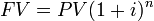
The future value (FV) measures the nominal future sum of money that a given sum of money is “worth” at a specified time in the future assuming a certain interest rate, or more generally, rate of return. The FV is calculated by multiplying the present value by the accumulation function. The value does not include corrections for inflation or other factors that affect the true value of money in the future. The process of finding the FV is often called capitalization.

On the other hand, the present value (PV) is the value on a given date of a payment or series of payments made at other times. The process of finding the PV from the FV is called discounting .

PV and FV are related, which reflects compounding interest ( simple interest has n multiplied by i, instead of as the exponent). Since it’s really rare to use simple interest, this formula is the important one.

PV and FV vary directly: when one increases, the other increases, assuming that the interest rate and number of periods remain constant.

The interest rate (or discount rate) and the number of periods are the two other variables that affect the FV and PV. The higher the interest rate, the lower the PV and the higher the FV. The same relationships apply for the number of periods. The more time that passes, or the more interest accrued per period, the higher the FV will be if the PV is constant, and vice versa.

The formula implicitly assumes that there is only a single payment. If there are multiple payments, the PV is the sum of the present values of each payment and the FV is the sum of the future values of each payment.

Calculating Perpetuities

The present value of a perpetuity is simply the payment size divided by the interest rate and there is no future value.

Perpetuities are a special type of annuity; a perpetuity is an annuity that has no end, or a stream of cash payments that continues forever. Essentially, they are ordinary annuities, but have no end date. There aren’t many actual perpetuities, but the United Kingdom has issued them in the past.

Since there is no end date, the annuity formulas we have explored don’t apply here. There is no end date, so there is no future value formula. To find the FV of a perpetuity would require setting a number of periods which would mean that the perpetuity up to that point can be treated as an ordinary annuity.

There is, however, a PV formula for perpetuities. The PV is simply the payment size (A) divided by the interest rate (r). Notice that there is no n, or number of periods. More accurately, is what results when you take the limit of the ordinary annuity PV formula as n → ∞.

It is also possible that an annuity has payments that grow at a certain rate per period. The rate at which the payments change is fittingly called the growth rate (g). The PV of a growing perpetuity is represented as

. It is essentially the same as in except that the growth rate is subtracted from the interest rate. Another way to think about it is that for a normal perpetuity, the growth rate is just 0, so the formula boils down to the payment size divided by r.

Calculating Values for Different Durations of Compounding Periods

Finding the Effective Annual Rate (EAR) accounts for compounding during the year, and is easily adjusted to different period durations.

Sometimes, the units of the number of periods does not match the units in the interest rate. For example, the interest rate could be 12% compounded monthly, but one period is one year. Since the units have to be consistent to find the PV or FV, you could change one period to one month. But suppose you want to convert the interest rate into an annual rate. Since interest generally compounds, it is not as simple as multiplying 1% by 12 (1% compounded each month). This atom will discuss how to handle different compounding periods.

Effective Annual Rate

The effective annual rate (EAR) is a measurement of how much interest actually accrues per year if it compounds more than once per year. The EAR can be found through the formula in where i is the nominal interest rate and n is the number of times the interest compounds per year (for continuous compounding, see ). Once the EAR is solved, that becomes the interest rate that is used in any of the capitalization or discounting formulas.

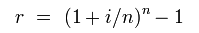
For example, if there is 8% interest that compounds quarterly, you plug.08 in for i and 4 in for n. That calculates an EAR of.0824 or 8.24%. You can think of it as 2% interest accruing every quarter, but since the interest compounds, the amount of interest that actually accrues is slightly more than 8%. If you wanted to find the FV of a sum of money, you would have to use 8.24% not 8%.

Solving for Present and Future Values with Different Compounding Periods

Solving for the EAR and then using that number as the effective interest rate in present and future value (PV/FV) calculations is demonstrated here. Luckily, it’s possible to incorporate compounding periods into the standard time-value of money formula. The equation in is the same as the formulas we have used before, except with different notation. In this equation, A(t) corresponds to FV, A₀ corresponds to Present Value, r is the nominal interest rate, n is the number of compounding periods per year, and t is the number of years.

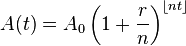
The equation follows the same logic as the standard formula. r/n is simply the nominal interest per compounding period, and nt represents the total number of compounding periods.

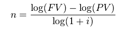
Solving for n

The last tricky part of using these formulas is figuring out how many periods there are. If PV, FV, and the interest rate are known, solving for the number of periods can be tricky because n is in the exponent. It makes solving for n manually messy. shows an easy way to solve for n. Remember that the units are important: the units on n must be consistent with the units of the interest rate (i).

 

Comparing Interest Rates

Variables, such as compounding, inflation, and the cost of capital must be considered before comparing interest rates.

The amount of interest you would have to pay on a loan or would earn on an investment is clearly an important consideration when making any financial decisions. However, it is not enough to simply compare the nominal values of two interest rates to see which is higher.

Effective Interest Rates

The reason why the nominal interest rate is only part of the story is due to compounding. Since interest compounds, the amount of interest actually accrued may be different than the nominal amount. The last section went through one method for finding the amount of interest that actually accrues: the Effective Annual Rate (EAR).

The EAR is a calculation that account for interest that compounds more than one time per year. It provides an annual interest rate that accounts for compounded interest during the year. If two investments are otherwise identical, you would naturally pick the one with the higher EAR, even if the nominal rate is lower.

Real Interest Rates

Interest rates are charged for a number of reasons, but one is to ensure that the creditor lowers his or her exposure to inflation. Inflation causes a nominal amount of money in the present to have less purchasing power in the future. Expected inflation rates are an integral part of determining whether or not an interest rate is high enough for the creditor.

The Fisher Equation is a simple way of determining the real interest rate, or the interest rate accrued after accounting for inflation. To find the real interest rate, simply subtract the expected inflation rate from the nominal interest rate.

For example, suppose you have the option of choosing to invest in two companies. Company 1 will pay you 5% per year, but is in a country with an expected inflation rate of 4% per year. Company 2 will only pay 3% per year, but is in a country with an expected inflation of 1% per year. By the Fisher Equation, the real interest rates are 1% and 2% for Company 1 and Company 2, respectively. Thus, Company 2 is the better investment, even though Company 1 pays a higher nominal interest rate.

Cost of Capital

Another major consideration is whether or not the interest rate is higher than your cost of capital. The cost of capital is the rate of return that capital could be expected to earn in an alternative investment of equivalent risk. Many companies have a standard cost of capital that they use to determine whether or not an investment is worthwhile.

In theory, a company will never make an investment if the expected return on the investment is less than their cost of capital. Even if a 10% annual return sounds really nice, a company with a 13% cost of capital will not make that investment.

Calculating Values for Fractional Time Periods

The value of money and the balance of the account may be different when considering fractional time periods.

Up to this point, we have implicitly assumed that the number of periods in question matches to a multiple of the compounding period. That means that the point in the future is also a point where interest accrues. But what happens if we are dealing with fractional time periods?

Compounding periods can be any length of time, and the length of the period affects the rate at which interest accrues.

Suppose the compounding period is one year, starting January1, 2012. If the problem asks you to find the value at June 1, 2014, there is a bit of a conundrum. The last time interest was actually paid was at January 1, 2014, but the time-value of money theory clearly suggests that it should be worth more in June than in January.

In the case of fractional time periods, the devil is in the details. The question could ask for the future value, present value, etc., or it could ask for the future balance, which have different answers.

Future/Present Value

If the problem asks for the future value (FV) or present value (PV), it doesn’t really matter that you are dealing with a fractional time period. You can plug in a fractional time period to the appropriate equation to find the FV or PV. The reasoning behind this is that the interest rate in the equation isn’t exactly the interest rate that is earned on the money. It is the same as that number, but more broadly, is the cost of not having the money for a time period. Since there is still a cost to not having the money for that fraction of a compounding period, the FV still rises.

Account Balance

The question could alternatively ask for the balance of the account. In this case, you need to find the amount of money that is actually in the account, so you round the number of periods down to the nearest whole number (assuming one period is the same as a compounding period; if not, round down to the nearest compounding period). Even if interest compounds every period, and you are asked to find the balance at the 6.9999^th period, you need to round down to 6. The last time the account actually accrued interest was at period 6; the interest for period 7 has not yet been paid.

If the account accrues interest continuously, there is no problem: there can’t be a fractional time period, so the balance of the account is always exactly the value of the money.

Loans and Loan Amortization

When borrowing money to be paid back via a number of installments over time, it is important to understand the time value of money and how to build an amortization schedule.

When lending money (or borrowing, depending on your perspective), it is common to have multiple payback periods over time (i.e. multiple, smaller cash flow installments to pay back the larger borrowed sum). In these situations, an amortization schedule will be created. This will determine how much will be paid back each period, and how many periods of repayment will be required to cover the principal balance. This must be agreed upon prior to the initial borrowing occurs, and signed by both parties.

Time Value of Money

Now if you add up all of the separate payments in an amortization schedule, you’ll find the total exceeds the amount borrowed. This is because amortization schedules must take into account the time value of money. Time value of money is a fairly simple concept at it’s core: a dollar today is worth more than a dollar tomorrow.

Why? Because capital can be invested, and those investments can yield returns. Lending your money to someone means incurring the opportunity cost of the other things you could do with that money. This gets even more drastic as the scale of capital increases, as the returns on capital over time are expressed in a percentage of the capital invested. Say you spend $100 on some stock, and turn 10% on that investment. You now have $110, a profit of $10. Say instead of only a $100, you put in $10,000. Now you have $11,000, a profit of $1,000.

Principle and Interest

As a result of this calculation, amortization schedules charge interest over time as a percentage of the principal borrowed. The calculation will incorporate the number of payment periods (n), the principal (P), the amortization payment (A) and the interest rate (r).

To make this a bit more realistic, let’s insert some numbers. Let’s say you find a dream house, at the reasonable rate of $100,000. Unfortunately, a bit of irresponsible borrowing in your past means you must pay 8% interest over a 30 year loan, which will be paid via a monthly amortization schedule (12 months x 30 years = 360 payments total). If you do the math, you should find yourself paying $734 per month 360 times. 360 x 734 will leave you in the ballpark of $264,000 in total repayment. that means you are paying more than 2.5 times as much for this house due to time value of money! This bit of knowledge is absolutely critical for personal financial decisions, as well as for high level business decisions.