A yield curve shows the relation between interest rate levels (or cost of borrowing) and the time to maturity.
Learning Objectives
Describe different yield curves
Key Takeaways
Key Points
- In finance the yield curve is a curve showing several yields or interest rates across different contract lengths for a similar debt contract.
- Based on the shape of the yield curve, we have normal yield curves, steep yield curves, flat or humped yield curves, and inverted yield curves.
- There are three main economic theories that attempt to explain different term structures of interest rates, namely the expectation hypothesis, the liquidity premium theory, and the segmented market hypothesis.
Key Terms
- Treasury bond: A United States Treasury security is a government debt issued by the United States Department of the Treasury through the Bureau of the Public Debt. Treasury securities are the debt financing instruments of the United States federal government, and they are often referred to simply as Treasuries. There are four types of marketable treasury securities: Treasury bills, Treasury notes, Treasury bonds, and Treasury Inflation Protected Securities (TIPS), in which Treasury bonds have the longest maturity, from 20 years to 30 years.
- treasury bill: A United States Treasury security is a government debt issued by the United States Department of the Treasury through the Bureau of the Public Debt. Treasury securities are the debt financing instruments of the United States federal government. They are often referred to simply as treasuries. There are four types of marketable treasury securities: Treasury bills, Treasury notes, Treasury bonds, and Treasury Inflation Protected Securities (TIPS), in which Treasury bills have the shortest maturity of one year or less.
- yield curve: the graph of the relationship between the interest on a debt contract and the maturity of the contract.
Overview
In finance the yield curve is a curve showing several yields or interest rates across different contract lengths (two month, two year, 20 year, etc…) for a similar debt contract. The curve shows the relation between the (level of) interest rate (cost of borrowing) and the time to maturity, known as the “term,” of the debt for a given borrower in a given currency. Based on the shape of the yield curve, we have normal yield curves, steep yield curves, flat or humped yield curves, and inverted yield curves.
The yield curve is normal meaning that yields rise as maturity lengthens (i.e., the slope of the yield curve is positive). This positive slope reflects investor expectations for the economy to grow in the future and, importantly, for this growth to be associated with a greater expectation that inflation will rise in the future rather than fall. This expectation of higher inflation leads to expectations that the central bank will tighten monetary policy by raising short term interest rates in the future to slow economic growth and dampen inflationary pressure.
Shapes of Curves
Sometimes, treasury bond yield averages higher than that of treasury bills (e.g. 20-year Treasury yield rises higher than the three-month Treasury yield). In situations when this gap increases, the economy is expected to improve quickly in the future. This type of steep yield curve can be seen at the beginning of an economic expansion (or after the end of a recession). Here, economic stagnation will have depressed short-term interest rates. However, rates begin to rise once the demand for capital is re-established by growing economic activity.
A flat yield curve is observed when all maturities have similar yields, whereas a humped curve results when short-term and long-term yields are equal and medium-term yields are higher than those of the short-term and long-term. A flat curve sends signals of uncertainty in the economy.
An inverted yield curve occurs when long-term yields fall below short-term yields. Why this would happen is that when lenders are seeking long-term debt contracts more aggressively than short-term debt contracts. The yield curve “inverts,” with interest rates (yields) being lower and lower for each longer periods of repayment so that lenders can attract long-term borrowing.
Theories
There are three main economic theories attempting to explain different term structures of interest rates. Two of the theories are extreme positions, while the third attempts to find a middle ground between the former two.
The expectation hypothesis of the term structure of interest rates is the proposition that the long-term rate is determined by the market’s expectation for the short-term rate plus a constant risk premium. Shortcomings of expectations theory is that it neglects the risks inherent in investing in bonds, namely interest rate risk and reinvestment rate risk.
The liquidity premium theory asserts that long-term interest rates not only reflect investors’ assumptions about future interest rates, but also include a premium for holding long-term bonds (investors prefer short term bonds to long term bonds), called the term premium or the liquidity premium. This premium compensates investors for the added risk of having their money tied up for a longer period, including the greater price uncertainty. Because of the term premium, long-term bond yields tend to be higher than short-term yields, and the yield curve slopes upward. Long term yields are also higher not just because of the liquidity premium, but also because of the risk premium added by the risk of default from holding a security over the long term.
In the segmented market hypothesis, financial instruments of different terms are not substitutable. As a result, the supply and demand in the markets for short-term and long-term instruments is determined largely independently. Prospective investors decide in advance whether they need short-term or long-term instruments. If investors prefer their portfolio to be liquid, they will prefer short-term instruments to long-term instruments. Therefore, the market for short-term instruments will receive a higher demand. Higher demand for the instrument implies higher prices and lower yield. This explains the stylized fact that short-term yields are usually lower than long-term yields. This theory explains the predominance of the normal yield curve shape. However, because the supply and demand of the two markets are independent, this theory fails to explain the observed fact that yields tend to move together (i.e., upward and downward shifts in the curve).
Using the Yield Curve to Estimate Interest Rates in the Future
Yield curves on bonds and government provided securities are correlative, and are useful in projected future rates.
Learning Objectives
Understand the conceptual implications of bond yield rates is they pertain to broader market interest rates
Key Takeaways
Key Points
- While the strict calculations involved in interest rate projections via bond yield curves come in a number of varieties (and complexities), it’s useful to note that there are strong correlations between the two.
- Yield curves combine the interest rate compounded over the duration of the debt security ‘s lifetime to demonstrate yield over time.
- The financial stress index uses bond yield rates to determine projected future yield curves, which can indicate a variety of economic predictions (such as recessions and interest rate changes).
- Market expectations theory uses existing projects for short-term interest rates based upon yield to project longer-term interest rates.
- The Heath-Jarrow-Morton Framework is a well-established norm for predicting interest rates based upon various inputs (including yield curves). Understanding the conceptual inputs to this model gives some scope as to interest rate derivation.
Key Terms
- recessions: Downturns in a given economic environment.
- yield curve: A curve that shows the compounded interest rate applied to the value of the security over its lifetime.
Defining the Yield Curve
For debt contracts, the overall duration of time of the debt security coupled with the interest rate compounded over that time frame will illustrate the overall yield of the security during its lifetime. This is referred to as a yield curve. When this is applied to U.S. treasury securities in respect to interest rates, useful information regarding projected interest rates in the future over time can be estimated. This is carefully monitored by many traders, and utilized as a point of comparison or benchmark for other investments (particularly valuation of bonds).

Relationship to the Business Cycle
Through assessing the slope of a yield curve on debt instruments such as governmental treasury bonds, investors can estimate the overall health of the economy in the future (i.e. inflation, interest rates, recessions, growth). Inverted yield curves are typically predictors of recession, while positively sloped yield curves indicate inflationary growth.
The Financial Stress Index
Defined as the rate of difference between a 10-year treasury bond rate and a 3-month treasury bond rate, the Financial Stress Index is a useful tool in projected future economic well-being. In fact, each of the recessionary periods since 1970 have demonstrated an inverted yield curve when subjected to Financial Stress Test just prior to that recessionary period.
Market Expectations (i.e. Pure Expectations)
When it comes to interest rates specifically, yield curves are useful constructs in projecting future behavior. The market expectations theory assumes that various maturities are perfect substitutes, and as a result the shape of the yield curve represents market expectations over time in relation to interest rates. In short, through investor expectations of what the 1-year interest rates will be next year, the current 2-year interest rate can be calculated as the compounding of this year’s 1-year interest rate by next year’s expected 1-year interest rate. Or, as an equation:
Heath-Jarrow-Morton Framework
When it comes to predicting future interest rates, the Heath-Jarrow-Morton framework is considered a standard approach. It focuses on modeling the evolution of the interest rate curve (instantaneous forward rate curve in particular). The equation itself is a rather evolved derivation, incorporating bond prices, forward rates, risk free rates, the Wiener process, Leibniz’s rule, and Fubini’s Theorem. While the details of this calculation are a bit outside the scope of discussion here, the equation can ultimately be described as:
For the sake of this discussion, it suffices to say that the input of existing yield curves is useful in projected future interest rates under a number of varying perspectives.
Macroeconomic Factors Influencing the Interest Rate
Taylor explained the rule of determining interest rates using three variables: inflation rate, GDP growth, and the real interest rate.
Learning Objectives
Describe how the nominal interest rate is influenced by inflation, output, and other economic conditions
Key Takeaways
Key Points
- In economics, the Taylor rule is a monetary-policy rule that stipulates how much the Central Bank should change the nominal interest rate in response to changes in inflation, output, or other economic conditions.
- If the inflationary expectation goes up, then so does the market interest rate and vice versa.
- If output gap is positive, it is called an “inflationary gap,” possibly creating inflation, signaling a increase in interest rates made by the Central Bank; if output gap is negative, it is called a “recessionary gap,” possibly signifying deflation and a reduction in interest rates.
Key Terms
- inflationary gap: An inflationary gap, in economics, is the amount by which the real gross domestic product, or real GDP, exceeds potential GDP.
- Real interest rate: The “real interest rate” is the rate of interest an investor expects to receive after allowing for inflation. It can be described more formally by the Fisher equation, which states that the real interest rate is approximately the nominal interest rate minus the inflation rate.
- Recessionary gap: An inflationary gap, in economics, is the amount by which the real Gross domestic product, or real GDP, is less than the potential GDP.
Interest Rate Overview
An interest rate is the rate at which interest is paid by a borrower for the use of money that they borrow from a lender in the market. The interest rates are influenced by macroeconomic factors. In economics, a Taylor rule is a monetary-policy rule that stipulates how much the Central Bank should change the nominal interest rate in response to changes in inflation, output, or other economic conditions. In particular, the rule stipulates that for each 1% increase in inflation, the Central Bank should raise the nominal interest rate by more than one percentage point.
Taylor Rule
According to Taylor’s original version of the rule, the nominal interest rate should respond to divergences of actual inflation rates from target inflation rates and of actual Gross Domestic Product (GDP) from potential GDP:
it = πt + r*t + απ(πt – π*t) + αy(yt – y*t)
In this equation, it is the target short-term nominal interest rate (e.g., the federal fund rates in the United States), πt is the rate of inflation as measured by the GDP deflator, π*t is the desired rate of inflation, r*t is the assumed equilibrium real interest rate, yt is the logarithm of real GDP, and y*t is the logarithm of potential output, as determined by a linear trend.
In other words, (πt – π*t)is inflation expectations that influence interest rates. Most economies generally exhibit inflation, meaning a given amount of money buys fewer goods in the future than it will now. The borrower needs to compensate the lender for this. If the inflationary expectation goes up, then so does the market interest rate and vice versa.
Output Gap
The GDP gap or the output gap is (yt – y*t). If this calculation yields a positive number, it is called an “inflationary gap” and indicates the growth of aggregate demand is outpacing the growth of aggregate supply (or high level of employment), possibly creating inflation, signaling an increase in interest rates made by the Central Bank; if the calculation yields a negative number it is called a “recessionary gap,” which is accompanied by a low employment rate, possibly signifying deflation and a reduction in interest rates.
In this equation, both απ and αy should be positive (as a rough rule of thumb, Taylor’s 1993 paper proposed setting απ =αy = 0.5). That is, the rule “recommends” a relatively high interest rate (a “tight” monetary policy) when inflation is above its target or when output is above its full-employment level, in order to reduce inflationary pressure. It recommends a relatively low interest rate (“easy” monetary policy) in the opposite situation to stimulate output.
Taylor explained the rule in simple terms using three variables: inflation rate, GDP growth, and the equilibrium real interest rate.
Licenses and Attributions
CC licensed content, Shared previously
- Curation and Revision. Provided by: Boundless.com. License: CC BY-SA: Attribution-ShareAlike
CC licensed content, Specific attribution
- Yield curve. Provided by: Wikipedia. License: CC BY-SA: Attribution-ShareAlike
- Term structure of interest rates. Provided by: Wikipedia. License: CC BY-SA: Attribution-ShareAlike
- Treasury bond. Provided by: Wikipedia. License: CC BY-SA: Attribution-ShareAlike
- treasury bill. Provided by: Wikipedia. License: CC BY-SA: Attribution-ShareAlike
- Yield curve israel shekel govt March 2008. Provided by: Wikimedia. License: CC BY-SA: Attribution-ShareAlike
- Yield to maturity. Provided by: Wikipedia. Located at: https://en.wikipedia.org/wiki/Yield_to_maturity. License: CC BY-SA: Attribution-ShareAlike
- Heath-Jarrow-Morton Framework. Provided by: Wikipedia. License: CC BY-SA: Attribution-ShareAlike
- Bond (finance). Provided by: Wikipedia. License: CC BY-SA: Attribution-ShareAlike
- Bond valuation. Provided by: Wikipedia. License: CC BY-SA: Attribution-ShareAlike
- Interest rate risk. Provided by: Wikipedia. License: CC BY-SA: Attribution-ShareAlike
- Yield curve. Provided by: Wikipedia. License: CC BY-SA: Attribution-ShareAlike
- Yield curve israel shekel govt March 2008. Provided by: Wikimedia. License: CC BY-SA: Attribution-ShareAlike
- USD_yield_curve_09_02_2005.JPG. Provided by: Wikimedia. Located at: https://upload.wikimedia.org/wikipedia/commons/1/18/USD_yield_curve_09_02_2005.JPG. License: CC BY-SA: Attribution-ShareAlike
- Interest rate. Provided by: Wikipedia. License: CC BY-SA: Attribution-ShareAlike
- Taylor rule. Provided by: Wikipedia. License: CC BY-SA: Attribution-ShareAlike
- Output gap. Provided by: Wikipedia. License: CC BY-SA: Attribution-ShareAlike
- inflationary gap. Provided by: Wikipedia. License: CC BY-SA: Attribution-ShareAlike
- Real interest rate. Provided by: Wikipedia. License: CC BY-SA: Attribution-ShareAlike
- Recessionary gap. Provided by: Wikipedia. License: CC BY-SA: Attribution-ShareAlike
- Yield curve israel shekel govt March 2008. Provided by: Wikimedia. License: CC BY-SA: Attribution-ShareAlike
- USD_yield_curve_09_02_2005.JPG. Provided by: Wikimedia. Located at: https://upload.wikimedia.org/wikipedia/commons/1/18/USD_yield_curve_09_02_2005.JPG. License: CC BY-SA: Attribution-ShareAlike
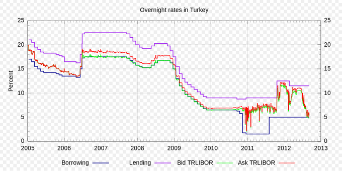
- Interest rates in Turkey. Provided by: Wikimedia. License: CC BY-SA: Attribution-ShareAlike
