6.3: Finding Probabilities for the Normal Distribution
Learning Objectives
- Find probabilities associated with the normal distribution.
Finding Probabilities with the Normal Table
Now that you have learned to assess the relative value of any normal value by standardizing, the next step is to evaluate probabilities. In other contexts, as mentioned before, we will first take the conventional approach of referring to a normal table, which tells the probability of a normal variable taking a value less than any standardized score z.
Click here to access the normal table.
Since normal curves are symmetric about their mean, it follows that the curve of z scores must be symmetric about 0. Since the total area under any normal curve is 1, it follows that the areas on either side of z = 0 are both .5. Also, according to the Standard Deviation Rule, most of the area under the standardized curve falls between z = -3 and z = +3.

The normal table outlines the precise behavior of the standard normal random variable Z, the number of standard deviations a normal value x is below or above its mean. The normal table provides probabilities that a standardized normal random variable Z would take a value less than or equal to a particular value z*.
These particular values are listed in the form *.* in rows along the left margins of the table, specifying the ones and tenths. The columns fine-tune these values to hundredths, allowing us to look up the probability of being below any standardized value z of the form *.**. Here is part of the table.
|
By construction, the probability P(Z < z*) equals the area under the z curve to the left of that particular value z*.

A quick sketch is often the key to solving normal problems easily and correctly.
Example
(a) What is the probability of a normal random variable taking a value less than 2.8 standard deviations above its mean? According to the table, P(Z < 2.8) = 0.9974 or 99.74%.
| z | 0.00 | 0.01 | 0.02 | 0.03 | 0.04 | 0.05 | 0.06 | 0.07 | 0.08 | 0.09 |
|---|---|---|---|---|---|---|---|---|---|---|
| 2.5 | 0.9938 | 0.9940 | 0.9941 | 0.9943 | 0.9945 | 0.9946 | 0.9948 | 0.9949 | 0.9951 | 0.9952 |
| 2.6 | 0.9953 | 0.9955 | 0.9956 | 0.9957 | 0.9959 | 0.9960 | 0.9961 | 0.9962 | 0.9963 | 0.9964 |
| 2.7 | 0.9965 | 0.9966 | 0.9967 | 0.9968 | 0.9969 | 0.9970 | 0.9971 | 0.9972 | 0.9973 | 0.9974 |
| 2.8 | 0.9974 | 0.9975 | 0.9976 | 0.9977 | 0.9977 | 0.9978 | 0.9979 | 0.9979 | 0.9980 | 0.9981 |
| 2.9 | 0.9981 | 0.9982 | 0.9982 | 0.9983 | 0.9984 | 0.9984 | 0.9985 | 0.9985 | 0.9986 | 0.9986 |
| 3.0 | 0.9987 | 0.9987 | 0.9987 | 0.9988 | 0.9988 | 0.9989 | 0.9989 | 0.9989 | 0.9990 | 0.9990 |

(b) What is the probability of a normal random variable taking a value lower than 1.47 standard deviations below its mean? P(Z < −1.47) = 0.0708, or 7.08%.
| z | 0.00 | 0.01 | 0.02 | 0.03 | 0.04 | 0.05 | 0.06 | 0.07 | 0.08 | 0.09 |
|---|---|---|---|---|---|---|---|---|---|---|
| -1.5 | 0.0668 | 0.0655 | 0.0643 | 0.0630 | 0.0618 | 0.0606 | 0.0594 | 0.0582 | 0.0571 | 0.0559 |
| -1.4 | 0.0808 | 0.0793 | 0.0778 | 0.0764 | 0.0749 | 0.0735 | 0.0721 | 0.0708 | 0.0694 | 0.0681 |
| -1.3 | 0.0968 | 0.0951 | 0.0934 | 0.0918 | 0.0901 | 0.0885 | 0.0869 | 0.0853 | 0.0838 | 0.0823 |
| -1.2 | 0.1151 | 0.1131 | 0.1112 | 0.1093 | 0.1075 | 0.1056 | 0.1038 | 0.1020 | 0.1003 | 0.0985 |

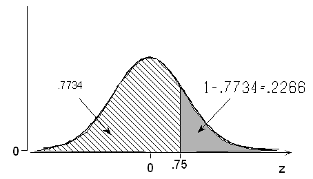
(c) What is the probability of a normal random variable taking a value more than 0.75 standard deviations above its mean?
The fact that the problem involves the word more rather than less should not be overlooked! Our normal table, like most, provides left-tail probabilities, and adjustments must be made for any other type of problem.
Method 1: By symmetry of the z curve centered on 0, P(Z > + 0.75) = P(Z < −0.75) = 0.2266.

Method 2: Because the total area under the normal curve is 1,
P(Z > + 0.75) = 1 − P(Z < + 0.75) = 1 − 0.7734 = 0.2266.

Note: Most students prefer to use Method 1, which does not require subtracting 4-digit probabilities from 1.
(d) What is the probability of a normal random variable taking a value between 1 standard deviation below and 1 standard deviation above its mean?
To find probabilities in between two standard deviations, we must put them in terms of the probabilities below. A sketch is especially helpful here:
P(−1 < Z < +1) = P(Z < +1) − P(Z < −1) = 0.8413 – 0.1587 = 0.6826.

Did I get this?
Comment
So far, we have used the normal table to find a probability, given the number (z) of standard deviations below or above the mean. The solution process involved first locating the given z value of the form *.** in the margins, then finding the corresponding probability of the form .**** inside the table as our answer. Now, in Example 2, a probability will be given and we will be asked to find a z value. The solution process involves first locating the given probability of the form .**** inside the table, then finding the corresponding z value of the form *.** as our answer.
Example
(a) The probability is .01 that a standardized normal variable takes a value below what particular value of z?
The closest we can come to a probability of .01 inside the table is .0099, in the z = -2.3 row and .03 column: z = -2.33. In other words, the probability is .01 that the value of a normal variable is lower than 2.33 standard deviations below its mean.
| z | .00 | .01 | .02 | .03 | .04 | .05 | .06 | .07 | .08 | .09 |
|---|---|---|---|---|---|---|---|---|---|---|
| -2.5 | .0062 | .0060 | .0059 | .0057 | .0055 | .0054 | .0052 | .0051 | .0049 | .0048 |
| -2.4 | .0082 | .0080 | .0078 | .0075 | .0073 | .0071 | .0069 | .0068 | .0066 | .0064 |
| -2.3 | .0107 | .0104 | .0102 | .0099 | .0096 | .0094 | .0091 | .0089 | .0087 | .0084 |
| -2.2 | .0139 | .0136 | .0132 | .0129 | .0125 | .0122 | .0119 | .0116 | .0113 | .0110 |
| -2.1 | .0179 | .0174 | .0170 | .0166 | .0162 | .0158 | .0154 | .0150 | .0146 | .0143 |

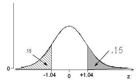
(b) The probability is .15 that a standardized normal variable takes a value above what particular value of z?
Remember that the table only provides probabilities of being below a certain value, not above. Once again, we must rely on one of the properties of the normal curve to make an adjustment.
Method 1: According to the table, .15 (actually .1492) is the probability of being below -1.04. By symmetry, .15 must also be the probability of being above +1.04.
| z | .00 | .01 | .02 | .03 | .04 | .05 | .06 | .07 | .08 | .09 |
|---|---|---|---|---|---|---|---|---|---|---|
| -1.2 | .1151 | .1131 | .1112 | .1093 | .1075 | .1056 | .1038 | .1020 | .1003 | .0985 |
| -1.1 | .1357 | .1335 | .1314 | .1292 | .1271 | .1251 | .1230 | .1210 | .1190 | .1170 |
| -1.0 | .1587 | .1562 | .1539 | .1515 | .1492 | .1469 | .1446 | .1423 | .1401 | .1379 |
| -0.9 | .1841 | .1814 | .1788 | .1762 | .1736 | .1711 | .1685 | .1660 | .1635 | .1611 |
| -0.8 | .2119 | .2090 | .2061 | .2033 | .2005 | .1977 | .1949 | .1922 | .1894 | .1867 |

Method 2: If .15 is the probability of being above the value we seek, then 1 – .15 = .85 must be the probability of being below the value we seek. According to the table, .85 (actually .8508) is the probability of being below +1.04.

In other words, we have found .15 to be the probability that a normal variable takes a value more than 1.04 standard deviations above its mean.
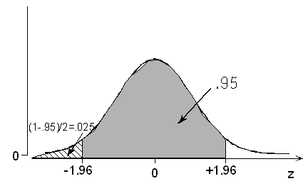
(c) The probability is .95 that a normal variable takes a value within how many standard deviations of its mean?
A symmetric area of .95 centered at 0 extends to values -z* and +z* such that the remaining (1 – .95) / 2 = .025 is below -z* and also .025 above +z*. The probability is .025 that a standardized normal variable is below -1.96. Thus, the probability is .95 that a normal variable takes a value within 1.96 standard deviations of its mean. Once again, the Standard Deviation Rule is shown to be just roughly accurate, since it states that the probability is .95 that a normal variable takes a value within 2 standard deviations of its mean.

Did I get this?
Comment
Our standard normal table, like most, only provides probabilities for z values between -3.49 and +3.49. The following example demonstrates how to handle cases where z exceeds 3.49 in absolute value.
Example
(a) What is the probability of a normal variable being lower than 5.2 standard deviations below its mean?
There is no need to panic about going “off the edge” of the normal table. We already know from the Standard Deviation Rule that the probability is only about (1 – .997) / 2 = .0015 that a normal value would be more than 3 standard deviations away from its mean in one direction or the other. The table provides information for z values as extreme as plus or minus 3.49: the probability is only .0002 that a normal variable would be lower than 3.49 standard deviations below its mean. Any more standard deviations than that, and we generally say the probability is approximately zero.
In this case, we would say the probability of being lower than 5.2 standard deviations below the mean is approximately zero:
P(Z < -5.2) = 0 (approx.)
(b) What is the probability of the value of a normal variable being higher than 6 standard deviations below its mean?
Since the probability of being lower than 6 standard deviations below the mean is approximately zero, the probability of being higher than 6 standard deviations below the mean must be approximately 1. P(Z > -6) = 1 (approx.)
(c) What is the probability of a normal variable being less than 8 standard deviations above the mean? Approximately 1. P(Z < +8) = 1 (approx.)
(d) What is the probability of a normal variable being greater than 3.5 standard deviations above the mean? Approximately 0. P(Z > +3.5) = 0 (approx.)
Working with Non-standard Normal Values
In a much earlier example, we wondered,
“How likely or unlikely is a male foot length of more than 13 inches?” We were unable to solve the problem, because 13 inches didn’t happen to be one of the values featured in the Standard Deviation Rule. Subsequently, we learned how to standardize a normal value (tell how many standard deviations below or above the mean it is) and how to use the normal table to find the probability of falling in an interval a certain number of standard deviations below or above the mean. By combining these two skills, we will now be able to answer questions like the one above.
Example
Male Foot Length
-
Male foot lengths have a normal distribution, with [latex]\mu=11, \sigma=1.5[/latex] inches. What is the probability of a foot length of more than 13 inches?

First, we standardize: [latex]\mathcal{z}=\frac{\mathcal{x}-\mu}{\sigma}=\frac{13-11}{1.5}=+1.33[/latex]; the probability that we seek, P(X > 13), is the same as the probabilityP(Z > +1.33) that a normal variable takes a value greater than 1.33 standard deviations above its mean.

This can be solved with the normal table, after applying the property of symmetry:
P(Z > +1.33) = P(Z < -1.33) = .0918. A male foot length of more than 13 inches is on the long side, but not too unusual: its probability is about 9%.
Comment:
We can streamline the solution in terms of probability notation. Since the standardized value for 13 is (13 – 11) / 1.5 = +1.33, we can write [latex]P(X>13)=P(Z>1.33)=P(Z<-1.33)=0.0918[/latex].
The first equality above holds because we subtracted the mean from a normal variable X and divided by its standard deviation, transforming it to a standardized normal variable that we call “Z.”
The second equality above holds by the symmetry of the standard normal curve around zero.
The last equality above was obtained from the normal table.
-
What is the probability of a male foot length between 10 and 12 inches?

The standardized values of 10 and 12 are, respectively, [latex]\frac{10-11}{1.5}=-0.67[/latex] and [latex]\frac{12-11}{1.5}=0.67[/latex]

P(-.67 < Z < +.67) = P(Z < +.67) – P(Z < -.67) = .7486 – .2514 = .4972.
Or, if you prefer the streamlined notation,
P(10<X<12)=P(−0.67<Z<+0.67)=P(Z<+0.67)−P(Z<−0.67)=0.7486−0.2514=0.4972.
Comment
By solving the above example, we inadvertently discovered the quartiles of a normal distribution! P(Z < -.67) = .2514 tells us that roughly 25%, or one quarter, of a normal variable’s values are less than .67 standard deviations below the mean. P(Z < +.67) = .7486 tells us that roughly 75%, or three quarters, are less than .67 standard deviations above the mean. And of course the median is equal to the mean, since the distribution is symmetric, the median is 0 standard deviations away from the mean.

Example
Length of a Human Pregnancy
Length (in days) of a randomly chosen human pregnancy is a normal random variable with μ=266,σ=16
-
Find Q1, the median, and Q3. Q1 = 266 – .67(16) = 255; median = mean = 266;
Q3 = 266 + .67(16) = 277. Thus, the probability is 1/4 that a pregnancy will last less than 255 days; 1/2 that it will last less than 266 days; 3/4 that it will last less than 277 days.

-
What is the probability that a randomly chosen pregnancy will last less than 246 days? Since (246 – 266) / 16 = -1.25, we write
P(X<246)=P(Z<−1.25)=0.1056
-
What is the probability that a randomly chosen pregnancy will last longer than 240 days? Since (240 – 266) / 16 = -1.63, we write
P(X>240)=P(Z>−1.63)=P(Z<+1.63)=0.9484
Since the mean is 266 and the standard deviation is 16, most pregnancies last longer than 240 days.
-
What is the probability that a randomly chosen pregnancy will last longer than 500 days?
Method 1: Common sense tells us that this would be impossible.
Method 2: The standardized value of 500 is (500 – 266) / 16 = +14.625. P(X>500)=P(Z>14.625)=0.
-
Suppose a pregnant woman’s husband has scheduled his business trips so that he will be in town between the 235th and 295th days. What is the probability that the birth will take place during that time? The standardized values are (235 – 266) / 16) = -1.94 and (295 – 266) / 16 = +1.81.
P(235<X<295)=P(−1.94<Z<+1.81)=P(Z<+1.81)−P(Z<−1.94)=0.9649−0.0262=0.9387
There is close to a 94% chance that the husband will be in town for the birth.
Learn by Doing
According to the College Board website, the scores on the math part of the SAT (SAT-M) in a certain year had a mean of 507 and standard deviation of 111. Assume that SAT scores follow a normal distribution.

