2.2: Measures of Central Tendency
Numerical Measures
The overall pattern of the distribution of a quantitative variable is described by its shape, center, and spread. By inspecting the histogram, we can describe the shape of the distribution, but as we saw, we can only get a rough estimate for the center and spread. A description of the distribution of a quantitative variable must include, in addition to the graphical display, a more precise numerical description of the center and spread of the distribution. In this section we will learn:
-
how to quantify the center and spread of a distribution with various numerical measures;
-
some of the properties of those numerical measures; and
-
how to choose the appropriate numerical measures of center and spread to supplement the histogram.
Measures of Center
Intuitively speaking, the numerical measure of center is telling us what is a “typical value” of the distribution.
The three main numerical measures for the center of a distribution are the mode, the mean and the median. Each one of these measures is based on a completely different idea of describing the center of a distribution. We will first present each one of the measures, and then compare their properties.
Mode
So far, when we looked at the shape of the distribution, we identified the mode as the value where the distribution has a “peak” and saw examples when distributions have one mode (unimodal distributions) or two modes (bimodal distributions). In other words, so far we identified the mode visually from the histogram.
Technically, the mode is the most commonly occurring value in a distribution. For simple datasets where the frequency of each value is available or easily determined, the value that occurs with the highest frequency is the mode.
Example
Best Actress Oscar Winners
We will continue with the Best Actress Oscar winners example. (To see the full dataset, Dataset_ Best Actress Oscar Winners (1970–2013)
To find the most commonly occurring, or modal, age, it is helpful to list the ages in a frequency table, which gives the following results:
|
The mode is 33, since it occurs the most times (6).
Example
World Cup Soccer
Often, we have large sets of data and use a frequency table to display the data more efficiently.
Data were collected from the last three World Cup soccer tournaments. A total of 192 games were played. The table below lists the number of goals scored per game (not including any goals scored in shootouts).
|
We can see that the most frequently occurring value is 2 goals (which occurred 51 times). Therefore, the mode for this set of data is 2.
Did I get this?
Here are the number of hours that 9 students spend on the computer on a typical day:
1 6 7 5 5 8 11 12 15
Mean
The mean is the average of a set of observations (i.e., the sum of the observations divided by the number of observations). If the n observations are [latex]x_1,x_2,...x_n[/latex], their mean, which we denote by [latex]\bar{\mathcal{x}}[/latex] (and read x-bar), is therefore: [latex]\bar{\mathcal{x}}=\frac{x1+x2+...+xn}{\mathcal{n}}[/latex]
Example
Best Actress Oscar Winners
Again we use the Best Actress Oscar winners example. (To see the full dataset, Dataset_ Best Actress Oscar Winners (1970–2013)
34 34 27 37 42 41 36 32 41 33 31 74 33 49 38 61 21 41 26 80 42 29 33 36 45 49 39 34 26 25 33 35 35 28 30 29 61 32 33 45 29 62 22 44
The mean age of the 32 actresses is [latex]\bar{\mathcal{x}}=\frac{34+34-27+...62+22+44}{44}=\frac{1687}{44}=38.3[/latex]
Note that the mean gives a measure of center that is higher than our approximation of the center from looking at the histogram (which was 35). The reason for this will be clear soon.
Example
World Cup Soccer
We now continue with the data from the last three World Cup soccer tournaments. A total of 192 games were played. The table below lists the number of goals scored per game (not including any goals scored in shootouts).
|
To find the mean number of goals scored per game, we would need to find the sum of all 192 numbers, then divide that sum by 192. Rather than add 192 numbers, we use the fact that the same numbers appear many times. For example, the number 0 appears 17 times, the number 1 appears 45 times, the number 2 appears 51 times, etc.
If we add up 17 zeros, we get 0. If we add up 45 ones, we get 45. If we add up 51 twos, we get 102. Repeated addition is multiplication.
Thus, the sum of the 192 numbers = 0(17) + 1(45) + 2(51) + 3(37) + 4(25) + 5(11) + 6(3) + 7(2) + 8(1) = 453.
The mean is 453/192 = 2.359.
This way of calculating a mean is sometimes referred to as a weighted average, since each value is “weighted” by its frequency. Note that, in this example, the values of 1, 2, and 3 are most heavily weighted.
Did I get this?
Median
The median M is the midpoint of the distribution. It is the number such that half of the observations fall above, and half fall below. To find the median:
-
Order the data from smallest to largest.
-
Consider whether n, the number of observations, is even or odd.
-
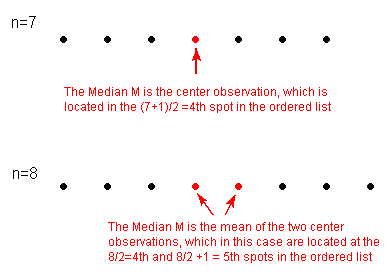
If n is odd, the median M is the center observation in the ordered list. This observation is the one “sitting” in the (n + 1)/2 spot in the ordered list.
-
If n is even, the median M is the mean of the two center observations in the ordered list. These two observations are the ones “sitting” in the n/2 and n/2 + 1 spots in the ordered list.
-
Example
Median (1)
For a simple visualization of the location of the median, consider the following two simple cases of n = 7 and n = 8 ordered observations, with each observation represented by a solid circle:

Example
Median (2)
To find the median age of the Best Actress Oscar winners, we first need to order the data. It would be useful, then, to use the stem plot, a diagram in which the data are already ordered.
Here n = 44 (an even number), so the median M, will be the mean of the two center observations. These are located at the n / 2 = 44 / 2 = 22nd and n / 2 + 1 = 44 / 2 + 1 = 23rd spots. Counting from the top, we find that:
-
the 22nd ranked observation is 34
-
the 23rd ranked observation is 35
Therefore, the median [latex]\mathcal{M}=\frac{(34+35)}{2}=34.5[/latex]

Did I get this?
Calculating mean, median, and mode
Explore this simulation activity to see how well you can calculate the mean and median for different data sets.
To view this interactive simulation in a separate window click here.
https://www.geogebra.org/m/KhKTscBY
CC BY-SA 3.0 by GeoGebra Group
Comparing the Mean and the Median
As we have seen, mean and the median, two of the common measures of center, each describe the center of a distribution of values in a different way. The mean describes the center as an average value, in which the actual values of the data points play an important role. The median, on the other hand, locates the middle value as the center, and the order of the data is the key to finding it.
To get a deeper understanding of the differences between these two measures of center, consider the following example.
Here are two datasets:
| Data set A → 64 65 66 68 70 71 73 |
| Data set B → 64 65 66 68 70 71 730 |
For dataset A, the mean is 68.1, and the median is 68. Looking at dataset B, notice that all of the observations except the last one are close together. The observation 730 is very large, and is certainly an outlier. In this case, the median is still 68, but the mean will be influenced by the high outlier, and shifted up to 162. The message that we should take from this example is:
The mean is very sensitive to outliers (because it factors in their magnitude), while the median is resistant to outliers.
Therefore:
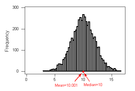
– For symmetric distributions with no outliers: ¯x is approximately equal to M.

– For skewed right distributions and/or datasets with high outliers: ¯x >M

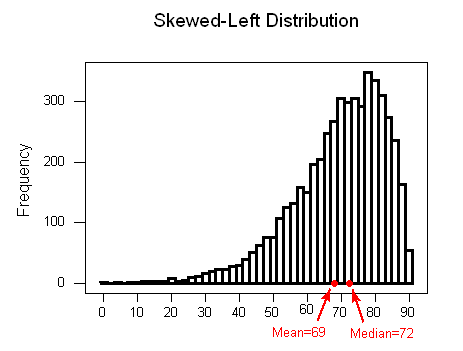
– For skewed left distributions and/or datasets with low outliers: ¯x <M

We will therefore use ¯x as a measure of center for symmetric distributions with no outliers. Otherwise, the median will be a more appropriate measure of the center of our data.
Did I get this?

Let’s Summarize
- The three main numerical measures for the center of a distribution are the mode, mean (¯x), and the median (M). The mode is the most frequently occurring value. The mean is the average value, while the median is the middle value.
- The mean is very sensitive to outliers (as it factors in their magnitude), while the median is resistant to outliers.
- The mean is an appropriate measure of center only for symmetric distributions with no outliers. In all other cases, the median should be used to describe the center of the distribution.
Prior to doing the checkpoint, you might want to do some additional problems that cover how to determine a median, mean, shape, relationship between a mean and median, and percentage of scores for a given value(s) from a histogram.

