6.2: Z-Scores
Finding Probabilities for a Normal Random Variable
As we saw, the Standard Deviation Rule is very limited in helping us answer probability questions, and basically limited to questions involving values that fall exactly 1, 2, and 3 standard deviations away from the mean. How do we answer probability questions in general? The key is the position of the value relative to the mean, measured in standard deviations.
We can approach the answering of probability questions two possible ways: a table and technology. In the next sections, you will learn how to use the “standard normal table,” and then how the same calculations can be done with technology.
Standardizing Values
The first step to assessing a probability associated with a normal value is to determine the relative value with respect to all the other values taken by that normal variable. This is accomplished by determining how many standard deviations below or above the mean that value is.
Example
Foot Length
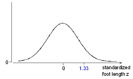
How many standard deviations below or above the mean male foot length is 13 inches? Since the mean is 11 inches, 13 inches is 2 inches above the mean. Since a standard deviation is 1.5 inches, this would be 2 / 1.5 = 1.33 standard deviations above the mean. Combining these two steps, we could write:
(13 in. – 11 in.) / (1.5 inches per standard deviation) = (13 – 11) / 1.5 standard deviations = +1.33 standard deviations.
In the language of statistics, we have just found the z-score for a male foot length of 13 inches to be z = +1.33. Or, to put it another way, we have standardized the value of 13. In general, the standardized value z tells how many standard deviations below or above the mean the original value is, and is calculated as follows:
z-score = (value – mean)/standard deviation
The convention is to denote a value of our normal random variable X with the letter “x.” Since the mean is written μ and the standard deviation σ, we may write the standardized value as
[latex]\mathcal{z}=\frac{\mathcal{x}-\mu}{\sigma}[/latex]
Notice that since σ is always positive, for values of x above the mean (μ), z will be positive; for values of x below μ, z will be negative.


Example
Standardizing Foot Measurements
Let’s go back to our foot length example, and answer some more questions.
(a) What is the standardized value for a male foot length of 8.5 inches? How does this foot length relate to the mean?
z = (8.5 – 11) / 1.5 = -1.67. This foot length is 1.67 standard deviations below the mean.
(b) A man’s standardized foot length is +2.5. What is his actual foot length in inches? If z = +2.5, then his foot length is 2.5 standard deviations above the mean. Since the mean is 11, and each standard deviation is 1.5, we get that the man’s foot length is: 11 + 2.5(1.5) = 14.75 inches.
z-scores also allow us to compare values of different normal random variables. Here is an example:
(c) In general, women’s foot length is shorter than men’s. Assume that women’s foot length follows a normal distribution with a mean of 9.5 inches and standard deviation of 1.2. Ross’ foot length is 13.25 inches, and Candace’s foot length is only 11.6 inches. Which of the two has a longer foot relative to his or her gender group?
To answer this question, let’s find the z-score of each of these two normal values, bearing in mind that each of the values comes from a different normal distribution.
Ross: z-score = (13.25 – 11) / 1.5 = 1.5 (Ross’ foot length is 1.5 standard deviations above the mean foot length for men).
Candace: z-score = (11.6 – 9.5) / 1.2 = 1.75 (Candace’s foot length is 1.75 standard deviations above the mean foot length for women).
Note that even though Ross’ foot is longer than Candace’s, Candace’s foot is longer relative to their respective genders.
To Sum Up … Part (c) illustrates how z-scores become crucial when you want to compare distributions.
Learn by Doing
The hourly salary rate for accountants at the “We are the Best Accounting Firm” follow a normal distribution, with a mean of $27 and a standard deviation of $4.
Did I get this?
Scores on the final exam in Professor Meyer’s statistics class follow a normal distribution, with a mean of 82 and a standard deviation of 5.

