10 Lesson 6 Stock
Similar to bonds, shares of common stock entitle investor owners to a portion of a company’s future earnings and cash flows. However, stocks differ significantly from bonds in how they are issued and managed by companies, the methodology used to calculate their values in public markets, and how they can generate income and eventual value for individual investors.
With common stock, there is no specific promise of how much cash investors will receive or when they will receive it. This differs from bond investments, which are valued entirely on the basis of their guaranteed timing of future cash flows to bondholders.
This means that with stocks, there are no maturity dates, face values, or coupon payment guarantees. It also means that stocks do not promise any specified cash flows in the form of coupons or a face value payment at some point in the future. Instead, stocks (only some, not all) may pay dividends. These dividends are declared after shares of stock have been issued by a company and then purchased by the investing public. Following a dividend declaration, the designated per-share amounts are paid to shareholders of record on a specified date, also determined by a company’s board.
Because stock investments carry no guarantee of payments to investors, they are far riskier than bonds and other forms of fixed-income investments.
While there are many reasons for an investor to choose to purchase common stock, three of the most
common reasons are
- to use stocks as instruments or repositories for maintaining value;
- to accumulate wealth over the term of the stock investment; and
- to earn income through capital gains and dividend payments.
As with any financial instrument, common stock purchases offer advantages and disadvantages to investors. Important advantages include the following:
- Returns through dividends and price appreciation of shares can be substantial.
- Stocks are a liquid form of investment and can be bought or sold within secondary markets relatively easily.
- Information about companies, markets, and important trends are widely published and readily available to the investing public.
These advantages are significant and lead many individuals to move into stock investments. Yet it is important to realize that stock has some significant disadvantages, which can include the following:
- General risk levels are greater than with bonds or other fixed-income investments.
- Timing the buy-and-sell transactions of stock can be tricky and may lead to losses or not taking full advantage of share price opportunities.
- Dividends (provided that the stock does indeed pay them, as not all do) are uncertain and subject to change based on decisions of company management.
We will discuss these topics in this chapter and cover many of the details regarding why corporations issue common stock and why investors purchase that stock.
 11.1
11.1
Multiple Approaches to Stock Valuation
Learning Outcomes
By the end of this section, you will be able to:
- Define and calculate a P/E (price-to-earnings) ratio given company data.
- Determine relative under- or overvaluation indicated by a P/E (price-to-earnings) ratio.
- Define and calculate a P/B (price-to-book) ratio given company data.
- Determine relative under- or overvaluation indicated by a P/B (price-to-book) ratio.
- Define and detail alternative valuation multipliers, including P/S (price-to-sales) ratio, P/CF (price-to-cash- flow) ratio, and dividend yield.
The Price-to Earnings (P/E) Ratio
Experienced investors use a number of different methods to evaluate information on companies and their common stock before deciding on any potential purchase. One of the most popular techniques used by investors and analysts is to study a company’s financial statements in order to uncover basic fundamental information on the company. This involves calculating a number of financial ratios that help identify trends, bringing elements of operational performance to light and allowing for clearer analysis and evaluation.
A well-proven analytical approach for investors to use in evaluating common stock is to review the overall market value of the company that issues a stock. One of the most consistently used calculations in this analysis, which has important applications in company and common stock evaluation, is the price-to-earnings (P/E) ratio.
The P/E ratio is computed using the following formula:

The P/E ratio is extremely useful to analysts in that it shows the expectations of the market. Essentially, the P/E ratio is representative of the price an investor must pay for every unit of current (or future) corporate earnings.
Bottom-line earnings are a critical factor in valuing common stock. Investors will always want to know how profitable a company is now as well as how profitable it will be in the future. When a company’s bottom line remains relatively flat over a period of time, leaving earnings per share (EPS) relatively unchanged, the P/E ratio can be interpreted as the payback period for the original amount paid for each share of common stock.
For example, the common stock price of Cameo Corp. is currently at $24.00 a share, and its EPS for the year is

$4.00. Cameo’s P/E ratio is calculated as

This ratio would typically be expressed in the form . Essentially, this means that investors are willing to pay up to six dollars for every one dollar of earnings. It can also be stated that Cameo stock is currently trading at a multiple of six.
The P/E ratio is typically expressed in two primary ways. The first is as a metric listed by most finance websites and often carries the notation P/E (ttm). This refers to the Wall Street acronym for “trailing 12 months” and signals the company’s operating performance over the past 12 months.
Another form of the P/E ratio is known as the forward (or leading) P/E. This uses future earnings projections rather than actual trailing amounts. The leading P/E, sometimes called the estimated price to earnings, is useful for comparing current earnings to future earnings and helps provide a clearer picture of what earnings may look like, assuming there are no major changes in the company’s operations or accounting treatments.
Referring back to our calculation for Cameo Corp. above, because the current EPS was used in the calculation, this ratio would be classified as a trailing P/E ratio. If we had used an estimated or projected EPS as the denominator in the calculation, it would then be considered a leading P/E ratio.
Analyzing a company’s P/E ratio alone or within a vacuum will actually tell an analyst very little. It is only when a company’s P/E is compared to historical P/E ratios or the P/E ratios of other companies in the same industry that it becomes a useful tool for analysis. One of the most important benefits of using comparative P/E ratios is that they can standardize stocks with different prices and various earnings levels.


 Generally speaking, it is very difficult to make any conclusions about a stand-alone stock value, such as whether a stock that has a ratio ofis a good buy at its current price or if a stock with a P/E ratio ofis too expensive, without performing any relevant comparisons or further analysis.
Analysts have many different ways to interpret P/E ratio data. One of the most common interpretations is that firms with high P/E ratios should be growth companies. Also, a high P/E ratio could mean that a stock’s price is high relative to earnings and possibly overvalued. This could signal a possible undesired downward adjustment in market price in the future.
We can extrapolate from the argument above to put forward the idea that stocks with low P/E ratios should be stabler, more mature organizations. A low P/E might indicate that the current stock price is low relative to earnings and that there may be an opportunity to take advantage of upward price movements and potential investment gains through stock price appreciation.
While this information is often very useful for evaluating stocks and making investment decisions, caution must always be used, as a current stock price may simply be out of line with the company’s earning potential, which would mean that price adjustments are likely to occur in the short term. This is why experienced analysts and investors will use multiple evaluation techniques when conducting stock analysis and evaluation and not rely solely on insights provided by a single set of facts or one form of statistical measurement.
The Price-to-Book (P/B) Ratio
Another financial ratio commonly used by investors and analysts is the price-to-book (P/B) ratio, also called the market-to-book (M/B) ratio. This is a financial metric used to evaluate a company’s current market value relative to its book value.
The market value, or market capitalization, of a company is defined as the current price of all its outstanding shares of common stock. This is essentially equal to the total value of the company as perceived by the market. For all intents and purposes, the book value is representative of the residual of a company after it has liquidated all assets and paid off all of its liabilities.
Book value can be determined by performing some financial analysis on a company’s balance sheet. Essentially, analysts will use the P/B ratio to compare a business’s available net assets relative to the current sales price of its stock. The price-to-book-value ratio formula is


One of the primary uses of the P/B ratio is to understand market perceptions of a particular stock’s value. It is often the metric of choice for evaluating financial services firms such as real estate firms, insurance companies, and investment trusts. The P/B ratio has a notable shortcoming, however, in that it does not evaluate companies that have a high level of intangible assets such as patents, trademarks, and copyrights.
 Ultimately, this ratio will tell an analyst exactly how much potential investors are willing to pay for each dollar of asset value. The PB(M/B) ratio is computed by dividing the current closing price of the stock by the company’s current book value per share, which is calculated by either of the following two equations:


Net book value is equal to net assets, or the total assets minus the total liabilities of the company.
Analysts often consider a low P/B ratio (less than 1) to indicate that a stock is undervalued and a higher ratio (greater than 1) to mean that a stock is overvalued. A low ratio may be an indication that something is wrong with the company or that an investor may be paying too much for any residual value should the company be liquidated.
However, many market experts will argue the exact opposite of the above interpretations. Because of these discrepancies in interpretation and overall variance of opinion, the use of alternate stock valuation metrics, either in addition to or in place of the P/B ratio, is always worth exploring.
In conclusion, the P/B ratio can help a company understand if its net assets are comparable to the market price of its stock. However, as with the P/E ratio, it is always a good idea to compare P/B ratios of companies within the same industry and use them in conjunction with other metrics and analytical methodologies.
LINK TO LEARNINGPrice-to-Earnings Ratio and Price-to-Book RatioTwo videos cover the price-to-earnings (P/E) ratio (https://openstax.org/r/price-to-earnings) and the price- to-book (P/B) ratio (https://openstax.org/r/price-to-book_ratio). These are excellent introductory videos that will provide you with helpful information on what these ratios represent and how they can be used in stock valuation.
Alternative Multipliers
There are two main types of valuation metrics multiples used to value common stock. These are equity multiples and enterprise value (EV) multiples. Additionally, there are two primary methods by which to perform analysis using these multiples. These methods are comparable company analysis (comps) and precedent transaction analysis (precedents).
Experienced financial analysts advocate the use of multiples in valuation analysis for a number of reasons, the most important being that they help generate realistic and sound judgments of enterprise values (total company values), they are relatively easy to use and interpret, and they can provide helpful information on a company’s overall financial condition when used appropriately.
However, it should be noted that simplicity may have some important disadvantages. When such complex information is reduced to a single equation or final value, it can easily be misunderstood, and the influence of important factors may be masked or lost in the evaluation process.
What’s more, the calculation of multiples represents a snapshot in time for a firm and cannot easily show how a company grows or progresses. Thus, these calculations are only applicable to short-term analysis, not to long-term scenarios.
Equity Multiples
Equity multiples are especially useful for investment decisions when an investor aspires to minority positions in companies. Below are some common equity multiples used in valuation analyses.
The price-to-earnings (P/E) ratio, which we discussed earlier, is probably the most common equity multiple used in stock valuation because it is relatively simple to calculate and all necessary data are easily accessible by analysts and investors. The market-to-book (M/B), or price-to-book (P/B), ratio is also useful if assets primarily drive a company’s earnings. Again, it is computed as the proportion of share price to book value per share.
Dividend yield is another form of equity multiple and is primarily used when conducting comparisons between cash returns and investment types. Dividend yield is computed as the proportion of dividend per share to share price. The price-to-sales (P/S) ratio is an additional metric used for firms that are experiencing financial losses. The P/S ratio is often used for quick estimates and is computed as the proportion of share price to sales (or revenue) per share.
Another useful metric is the price-to-cash-flow (P/CF) ratio. The P/CF ratio is used to compare a company’s market value to its operating cash flow (or the company’s stock price per share to its operating cash flow per share). This measurement is suitable only in certain cases, such as when a company has substantial noncash expenses (e.g., depreciation or amortization). In some situations, companies may have positive cash flows but still show a bottom-line loss due to large noncash expenses. The P/CF ratio is helpful for arriving at a less distorted view of such a company’s value.
While these various metrics are important, a financial analyst must always consider that companies often operate under their own unique sets of circumstances that ultimately will influence many of these equity multiples.
Enterprise Value (EV) Multiples
 The following are some common EV multiples used in valuation analyses: Gordon growth model is as follows
EV multiples take an increasingly important role when value decisions surround recent mergers and acquisitions. Enterprise value (EV) is a measurement of the total value of a company. Companies often believe that EV offers a more accurate representation of a firm’s total value than a basic market capitalization method. Generally, EV is perceived to offer an aggregate value of the firm as an enterprise, which is a more comprehensive measurement (see Figure 11.2).
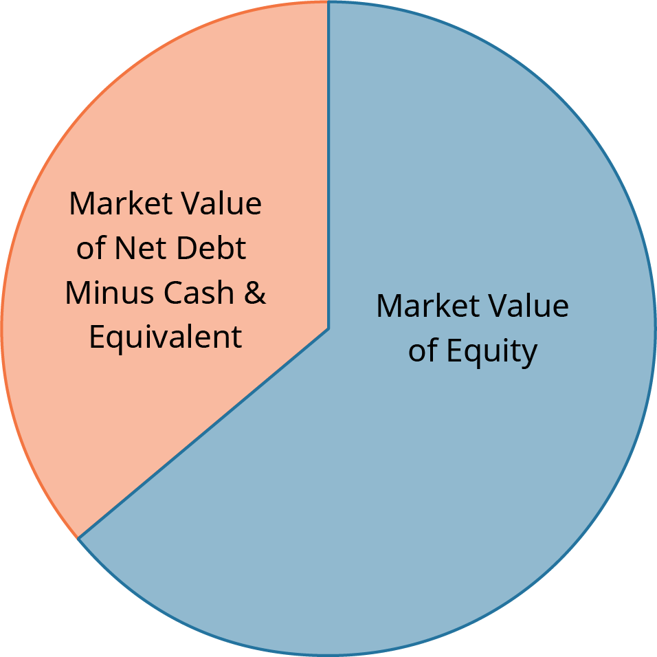
Figure 11.2 Enterprise Value: The Complete Picture
Following are two of the most common enterprise values metrics used in valuing companies and their common stock:
EV/Revenue (EV/R). Also called EV/Sales, EV/R is a valuation metric used to understand a company’s total valuation compared to its annual sales levels. EV/R can help provide an analyst with an idea of exactly how much investors pay for every dollar of a company’s sales revenue.
EV/R is considered a relatively crude metric but can be useful when analyzing companies that have different methods of revenue recognition. P/E ratios, for example, can be significantly affected by changes in the accounting policies of companies being evaluated. This is another reason why multiple metrics should be used in valuations.
Additionally, EV/R is a useful measure for companies that are consuming cash or experiencing financial losses. Such companies may be start-ups or emerging technology firms that have not fully matured and are still in a growth stage of development.
EV/EBIT. A firm’s earnings before interest and taxes (EBIT) is an indicator of its profitability before the effects of interest or taxes. EBIT is also referred to as operating earnings, operating profit, and profit before interest and tax.
- EV/EBITDA. EV/EBITDA is a ratio that compares a company’s enterprise value (EV) to its earnings before interest, taxes, depreciation, and amortization (EBITDA). EBITDA is often used by analysts as a substitute for cash flow and can be applied to capital analysis using tools such as net present value and internal rate of return. It is relatively easy to calculate, as all information required to compete the calculation is
available from any publicly traded company’s financial statements. Because of this, the EV/EBITDA ratio is a commonly used metric to compare the relative values of different businesses.
- EV/EBITDAR. Another form of valuation based on enterprise value is EV/EBITDAR. This metric divides enterprise value by earnings before interest, tax, depreciation, amortization, and rental costs (EBITDAR). This multiple is used in businesses that have substantial rental and lease expenses, such as hotel chains and airlines. Capital investment can differ significantly for these firms, and when assets are leased, these companies tend to have artificially lower debt and operating income compared to firms that actually own their assets.
EV/Capital Employed. The EV-to-capital employed ratio is a measure of enterprise value compared to the level of capital used by a business. For example, a business with a large capital basis is bound to carry a large enterprise value simply due to its large capital holdings.
Final Thoughts on Valuation Ratios and Multiples
There are many equity and enterprise value multiples used in company valuation, but the discussions above cover those that are most commonly used. In any case, gaining a thorough understanding of each multiple and its related concepts can help analysts make better use of these metrics in their stock analysis and valuation efforts. Also, as discussed, it is important that analysts and technicians use multiple ratios and alternate measures for any evaluation of a company and its common stock. Not doing so will limit the ultimate interpretation of the results, can lead to incorrect conclusions, and may cause fundamental mistakes in overall investment strategy.
 LINK TO LEARNINGGraph of Historical P/E for S&P 500Look at the 90-year historical average P/E ratio of the S&P 500 (https://openstax.org/r/90-year_historical_average_P/E). When viewing this information on historical P/E ratios, think about the following:Note that the general trend for historical P/E ratios has been one of growth.Note that in May 2009, the P/E ratio reached a staggeringthe highest ratio in US history. This was primarily due to depressed earnings during the Great Recession.
11.2
Dividend Discount Models (DDMs)
Learning Outcomes
By the end of this section, you will be able to:
- Identify and use DDMs (dividend discount models).
- Define the constant growth DDM.
- List the assumptions and limitations of the Gordon growth model.
- Understand and be able to use the various forms of DDM.
- Explain the advantages and limitations of DDMs.
The dividend discount model (DDM) is a method used to value a stock based on the concept that its worth is the present value of all of its future dividends. Using the stock’s price, a required rate of return, and the value of the next year’s dividend, investors can determine a stock’s value based on the total present value of future dividends.
This means that if an investor is buying a stock primarily based on its dividend, the DDM can be a useful tool to determine exactly how much of the stock’s price is supported by future dividends. However, it is important to
understand that the DDM is not without flaws and that using it requires assumptions to be made that, in the end, may not prove to be true.
The Gordon Growth Model
The most common DDM is the Gordon growth model, which uses the dividend for the next year (D1), the required return (r), and the estimated future dividend growth rate (g) to arrive at a final price or value of the stock. The formula for the Gordon growth model is as follows:


This calculation values the stock entirely on expected future dividends. You can then compare the calculated price to the actual market price in order to determine whether purchasing the stock at market will meet your requirements.
LINK TO LEARNINGDividend Discount ModelWatch this short video on the dividend discount model (https://openstax.org/r/ short_video_on_the_dividend) and how it is used it in stock valuation and analysis.The Gordon growth model equation is presented and then applied to a sample problem to demonstrate how the DDM yields an estimated share price for the stock of any company.
Now that we have been introduced to the basic idea behind the dividend discount model, we can move on to cover other forms of DDM.
Zero Growth Dividend Discount Model
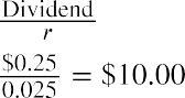
The zero growth DDM assumes that all future dividends of a stock will be fixed at essentially the same dollar value forever, or at least for as long as an individual investor holds the shares of stock. In such a case, the stock’s intrinsic value is determined by dividing the annual dividend amount by the required rate of return:

When examined closely, it can be seen that this is the exact same formula that is used to calculate the present value of a perpetuity, which is
For the purpose of using this formula in stock valuation, we can express this as


where PV is equal to the price or value of the stock, D represents the dividend payment, and r represents the required rate of return.
This makes perfect sense because a stock that pays the exact same dividend amount forever is no different from a perpetuity—a continuous, never-ending annuity—and for this reason, the same formula can be used to price preferred stock. The only factor that might alter the value of a stock based on the zero-growth model would be a change in the required rate of return due to fluctuations in perceived risk levels.
Example:
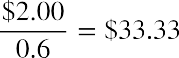
What is the intrinsic value of a stock that pays $2.00 in dividends every year if the required rate of return on similar investments in the market is 6%?
Solution:
We can apply the zero growth DDM formula to get

While this model is relatively easy to understand and to calculate, it has one significant flaw: it is highly unlikely that a firm’s stock would pay the exact same dollar amount in dividends forever, or even for an extended period of time. As companies change and grow, dividend policies will change, and it naturally follows that the payout of dividends will also change. This is why it is important to become familiar with other DDMs that may be more practical in their use.
Constant Growth Dividend Discount Model
As indicated by its name, the constant growth DDM assumes that a stock’s dividend payments will grow at a fixed annual percentage that will remain the same throughout the period of time they are held by an investor. While the constant growth DDM may be more realistic than the zero growth DDM in allowing for dividend growth, it assumes that dividends grow by the same specific percentage each year. This is also an unrealistic assumption that can present problems when attempting to evaluate companies such as Amazon, Facebook, Google, or other organizations that do not pay dividends. Constant growth models are most often used to value mature companies whose dividend payments have steadily increased over a significant period of time. When applied, the constant growth DDM will generate the present value of an infinite stream of dividends that are growing at a constant rate.
The constant growth DDM formula is


where D0 is the value of the dividend received this year, D1 is the value of the dividend to be received next year, g is the growth rate of the dividend, and r is the required rate of return.
As can be seen above, after simplification, the constant growth DDM formula becomes the Gordon growth model formula and works in the same way. Let’s look at some examples.
 THINK IT THROUGHConstant Growth DDM: Example 1If a stock is paying a dividend of $5.00 this year and the dividend has been steadily growing at 4% annually, what is the intrinsic value of the stock, assuming an investor’s required rate of return of 8%?Solution:Apply the constant growth DDM formula:Simplify to the Gordon growth model:

 THINK IT THROUGHConstant Growth DDM: Example 2If a stock is selling at $250 with a current dividend of $10, what would be the dividend growth rate of this stock, assuming a required rate of return of 12%?Solution:Apply the constant growth DDM formula:Simplify and continue the calculation:So, the growth rate is 7.69%.
LINK TO LEARNINGDividend Discount Model: A Complete Animated GuideIn this video for the Investing for Beginners course and podcast, Andrew Sather introduces the DDM, (https://openstax.org/r/Andrew_Sather_introduces_the_DDM) demonstrating both the constant growth DDM (Gordon growth model) and the two-stage DDM.
Variable or Nonconstant Growth Dividend Discount Model
Many experienced analysts prefer to use the variable (nonconstant) growth DDM because it is a much closer approximation of businesses’ actual dividend payment policies, making it much closer to reality than other forms of DDM. The variable growth model is based on the real-life assumption that a company and its stock value will progress through different stages of growth.
The variable growth model is estimated by extending the constant growth model to include a separate calculation for each growth period. Determine present values for each of these periods, and then add them all together to arrive at the intrinsic value of the stock. The variable growth model is more involved than other DDM methods, but it is not overly complex and will often provide a more realistic and accurate picture of a stock’s true value.
As an example of the variable growth model, let’s say that Maddox Inc. paid $2.00 per share in common stock dividends last year. The company’s policy is to increase its dividends at a rate of 5% for four years, and then the growth rate will change to 3% per year from the fifth year forward. What is the present value of the stock if the required rate of return is 8%? The calculation is shown in Table 11.1.
Table 11.1 Value of Stock with 8% Required Rate of Return
Note:

The value of Maddox stock in this example would be $43.25 per share.
Two-Stage Dividend Discount Model
The two-stage DDM is a methodology used to value a dividend-paying stock and is based on the assumption of two primary stages of dividend growth: an initial period of higher growth and a subsequent period of lower, more stable growth.
The two-stage DDM is often used with mature companies that have an established track record of making residual cash dividend payments while experiencing moderate rates of growth. Many analysts like to use the two-stage model because it is reasonably grounded in reality. For example, it is probably a more reasonable assumption that a firm that had an initial growth rate of 10% might see its growth drop to a more modest level of, say, 5% as the company becomes more established and mature, rather than assuming that the firm will maintain the initial growth rate of 10%. Experts tend to agree that firms that have higher payout ratios of dividends may be well suited to the two-stage DDM.
As we have seen, the assumptions of the two-stage model are as follows:
- The first period analyzed will be one of high initial growth.
- This stage of higher growth will eventually transition into a period of more mature, stable, and sustainable growth at a lower rate than the initial high-growth period.
- The dividend payout ratio will be based on company performance and the expected growth rate of its operations.
Let’s use an example. Lore Ltd. estimates that its dividend growth will be 13% per year for the next five years. It will then settle to a sustainable, constant, and continuing rate of 5%. Let’s say that the current year’s dividend is $14 and the required rate of return (or discount rate) is 12%. What is the current value of Lore Ltd. stock?
Step 1:
First, we will need to calculate the dividends for each year until the second, stable growth rate phase is reached. Based on the current dividend value of $14 and the anticipated growth rate of 13%, the values of dividends (D1, D2, D3, D4, D5) can be determined for each year of the first phase. Because the stable growth rate is achieved in the second phase, after five years have passed, if we assume that the current year is 2021, we can lay out the profile for this stock’s dividends through the year 2026, as per Figure 11.3.
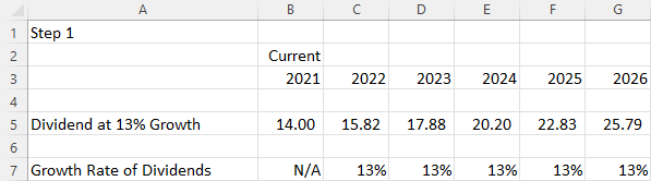
Figure 11.3 Profile of Stock Dividend through 2026
Next, we apply the DDM to determine the terminal value, or the value of the stock at the end of the five-year high-growth phase and the beginning of the second, lower growth-phase.
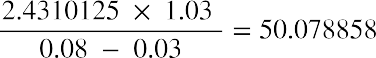
We can apply the DDM formula at any point in time, but in this example, we are working with a stock that has constant growth in dividends for five years and then decreases to a lower growth rate in its secondary phase. Because of this timing and dividend structure, we calculate the value of the stock five years from now, or the terminal value. Again, this is calculated at the end of the high-growth phase, in 2026. By applying the constant growth DDM formula, we arrive at the following:


The terminal value can be calculated by applying the DDM formula in Excel, as seen in Figure 11.4 and Figure
11.5. The terminal value, or the value at the end of 2026, is $386.91.
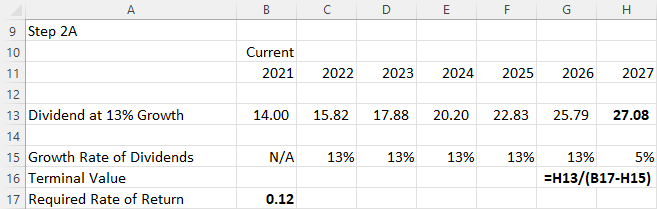
Figure 11.4 Terminal Value at the End of 2026 (Showing Formula)
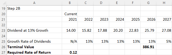
Figure 11.5 Terminal Value at the End of 2026
Next, we find the PV of all paid dividends that occur during the high-growth period of 2022–2026. This is shown in Figure 11.6. Our required rate of return (discount rate) is 12%.
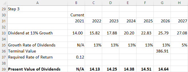
Figure 11.6 Present Value of All Paid Dividends, 2022–2026
Next, we calculate the PV of the single lump-sum terminal value:


Remember that due to the sign convention, either the FV must be entered as a negative value or, if entered as a positive value, the resulting PV will be negative. This example shows the former.
Step 5:
Our next step is to find the current fair (intrinsic) value of the stock, which comprises the PV of all future dividends plus the PV of the terminal value. This is represented in the following formula, with all factors shown in Figure 11.7:


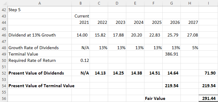
Figure 11.7 Fair Value of the Stock
So, we end up with a total current fair value of Lore Ltd. stock of $291.44 (due to Excel’s rounding), although the sum can also be calculated as shown below:


LINK TO LEARNINGDetermining Stock ValueTake a few minutes to review this video, which covers methods used to determine stock value (https://openstax.org/r/covers_methods_used_to_determine_stock_value) when dividend growth is nonconstant.
Advantages and Limitations of DDMs
Some of the primary advantages of DDMs are their basis in the sound logic of present value concepts, their consistency, and the implication that companies that pay dividends tend to be mature and stable entities. Also, because the model is essentially a mathematical formula, there is little room for misinterpretation or subjectivity. As a result of these advantages, DDMs are a very popular form of stock evaluation that most analysts show faith in.
Because dividends are paid in cash, companies may keep making their dividend payments even when doing so is not in their best long-term interests. They may not want to manipulate dividend payments, as this can directly lead to stock price volatility. Rather, they may manipulate dividend payments in the interest of buoying up their stock price.
To further illustrate limitations of DDMs, let’s examine the Concepts in Practice case.
CONCEPTS IN PRACTICELimitations of DDMsA major limitation of the dividend discount model is that it cannot be used to value companies that do not pay dividends. This is becoming a growing trend, particularly for young high-tech companies. Warren Buffett, CEO of Berkshire Hathaway, has stated that companies are usually better off if they take their excess funds and reinvest them into infrastructure, evolving technologies, and other profitable ventures. The payment of dividends to shareholders is “almost a last resort for corporate management,”1 says Buffett, and cash balances should be invested in “projects to become more efficient, expand territorially, extend and improve product lines or . . . otherwise widen the economic moat separating the company from its competitors.”2 Berkshire follows this practice of reinvesting cash rather than paying dividends, as do tech companies such as Amazon, Google, and Biogen.3 So, rather than receiving cash dividends, stockholders of these companies are rewarded by seeing stock price appreciation in their investments and ultimately large capital gains when they finally decide to sell their shares.The sensitivity of assumptions is also a drawback of using DDMs. The fair price of a stock can be highly sensitive to growth rates and the required rates of return demanded by investors. A single percentage point change in either of these two factors can have a dramatic impact on a company’s stock, potentially changing it by as much as 10 to 20%.
- Dan Caplinger. “Why Don’t These Winning Stocks Pay Dividends?” The Motley Fool. Updated October 3, 2018. https://www.fool.com/investing/general/2015/03/01/why-dont-these-winning-stocks-pay-dividends.aspx
- The Motley Fool. “Why Warren Buffet’s Berkshire Hathaway Won’t Pay a Dividend in 2015.” Nasdaq. November 16, 2014. https://www.nasdaq.com/articles/why-warren-buffetts-berkshire-hathaway-wont-pay-dividend-2015-2014-11-16.
- Caplinger, “Why Don’t These Winning Stocks Pay Dividends?” The Motley Fool.
Finally, the results obtained using DDMs may not be related to the results of a company’s operations or its profitability. Dividend payments should theoretically be tied to a company’s profitability, but in some instances, companies will make misguided efforts to maintain a stable dividend payout even through the use of increased borrowing and debt, which is not beneficial to an organization’s long-term financial health.(sources: www.wallstreetmojo.com/dividend-discount-model/; pages.stern.nyu.edu/~adamodar/pdfiles/ valn2ed/ch13d.pdf; www.managementstudyguide.com/disadvantages-of-dividend-discount-model.htm)
Stock Valuation with Changing Growth Rates and Time Horizons
Before we move on from our discussion of dividend discount models, let’s work through some more examples of how the DDM can be used with a number of different scenarios, changing growth rates, and time horizons.
As we have seen, the value or price of a financial asset is equal to the present value of the expected future cash flows received while maintaining ownership of the asset. In the case of stock, investors receive cash flows in the form of dividends from the company, plus a final payout when they decide to relinquish their ownership rights or sell the stock.
Let’s look at a simple illustration of the price of a single share of common stock when we know the future dividends and final selling price.
Problem:
Steve wants to purchase shares of Old Peak Construction Company and hold these common shares for five years. The company will pay $5.00 annual cash dividends per share for the next five years.
At the end of the five years, Steve will sell the stock. He believes that he will be able to sell the stock for $25.00 per share. If Steve wants to earn 10% on this investment, what price should he pay today for this stock?
Solution:
The current price of the stock is the discounted cash flow that Steve will receive over the next five years while holding the stock. If we let the final price represent a lump-sum future value and treat the dividend payments as an annuity stream over the next five years, we can apply the time value of money concepts we covered in earlier chapters.
Method 1: Using an Equation


Method 2: Using a Financial Calculator
 We can also use a calculator or spreadsheet to find the price of the stock (see Table 11.2).
|
Description |
Enter |
Display |
|
|
1 |
Clear calculator register |
CE/C |
|
|
2 |
Enter number of periods (5) |
5 N |
N =5.00 |
|
3 |
Enter rate of return or interest rate (10%) |
10 I/Y |
I/Y =10.00 |
|
4 |
Enter eventual sales price ($25) |
25 FV |
FV =25.00 |
|
5 |
Enter dividend amount ($5) |
5 PMT |
PMT =5.00 |
|
6 |
Compute present value |
CPT PV |
PV =– 34.47 |
Table 11.2 Calculator Steps for Finding the Price of the Stock4
The stock price is calculated as $34.47.
Note that the value given is expressed as a negative value due to the sign convention used by financial calculators. We know the actual stock value is not negative, so we can just ignore the minus sign.
In cases such as the above, we find the present value of a dividend stream and the present value of the lump- sum future price. So, if we know the dividend stream, the future price of the stock, the future selling date of the stock, and the required return, it is possible to price stocks in the same manner that we price bonds.
Method 3: Using Excel
Figure 11.8 shows a spreadsheet setup in Excel to reach a solution to this problem.
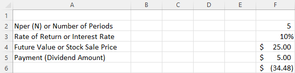
Figure 11.8 Excel Solution for Finding the Price of the Stock
Due to the sign convention in Excel, we can ignore the parentheses around the solution, which indicate a negative value. Therefore, the price is $34.48. The Excel command used in cell F6 to calculate present value is as follows:
=PV(rate,nper,pmt,[fv],[type])
Finding Stock Price with Constant Dividends Example 1:
Four Seasons Resorts pays a $0.25 dividend every quarter and will maintain this policy forever. What price should you pay for one share of common stock if you want an annual return of 10% on your investment?
Solution:


You can restate your annual required rate of 10% as a quarterly rate of. Apply the quarterly dividend amount and the quarterly rate of return to determine the price:
- The specific financial calculator in these examples is the Texas Instruments BA II PlusTM Professional model, but you can use other financial calculators for these types of calculations.


 Even though we anticipate that companies will be in business “forever,” we are not going to own a company’s stock forever. Therefore, the dividend stream to which we would have legal claim is only for that period of the company’s life during which we own the stock. We need to modify the dividend model to account for a finite period when we will sell the stock at some future time. This modification brings us from an infinite to a finite dividend pricing model, which we will use to price a finite amount of dividends and the future selling price of the stock. We will maintain a constant dividend assumption. Let’s assume we will hold a share in a company that pays a $1 dividend for 20 years and then sell the stock.
Method 1: Using an Equation
The dividend pricing model under a finite horizon is a concept we have seen earlier. It is a simple present value annuity stream application:


We now need to determine the selling price that we would get in 20 years if we were to sell the stock to someone else at that time. What would a willing buyer give us for the stock 20 years from now? This price is difficult to estimate, so for the sake of this exercise, we will assume that the price in 20 years will be $30. So, what is the present value of the price in 20 years with a 10% discount rate? Again, this is just a simple application of the PV formula we covered earlier in the text:


We can now price the stock as if it were a bond with a dividend stream of 20 years, a sales price in 20 years, and a required return of 10%:
- The dividend stream is analogous to the coupon payments.
- The sales price is analogous to the bond’s principal.
- The 20-year investment horizon is analogous to the bond’s maturity date.
- The required return is analogous to the bond’s yield.
Carrying on with the PV calculations, we have


Method 2: Using a Financial Calculator
We can also use a calculator or spreadsheet to find the price of the stock using constant dividends (see Table 11.3).
|
Description |
Enter |
Display |
||
|
|
Clear calculator register |
CE/C |
|
0.00 |
Table 11.3 Calculator Steps for Finding the Price of Stock Using Constant Dividends
|
|
Description |
Enter |
|
|
2 |
Enter number of periods (20) |
20 N |
N =20.00 |
|
3 |
Enter rate of return or interest rate (10%) |
10 I/Y |
I/Y =10.00 |
|
4 |
Enter eventual sales price (30) |
30 FV |
FV =30.00 |
|
5 |
Enter dividend amount ($1) |
1 PMT |
PMT =1.00 |
|
6 |
Compute present value |
CPT PV |
PV =−12.97 |
Table 11.3 Calculator Steps for Finding the Price of Stock Using Constant Dividends
The stock price resulting from the calculation is $12.97.
Method 3: Using Excel
This same problem can be solved using Excel with a setup similar to that shown in Figure 11.9.
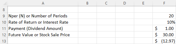
Figure 11.9 Excel Solution for Finding the Price of Stock Using Constant Dividends
Once again, we can ignore the negative indicator that is generated by the Excel sign convention because we know that the stock will not have a negative value 20 years from now. Therefore, the price is $12.97. The Excel command used in cell F13 to calculate present value is as follows:
Example 2:
=PV(rate,nper,pmt,[fv],[type])


 Let’s look at an example and estimate current stock price given a 10.44% constant growth rate of dividends forever and a desired return on the stock of 13.5%. We will assume that the current stock owner has just received the most recent dividend, D0, and the new buyer will receive all future cash dividends, beginning with D1. This part of the setup of the model is important because the price reflects all future dividends, starting with D1, discounted back to today. (Price0 refers to the price at time zero, or today.) The first dividend the buyer would receive is one full period away. Using the discounted cash flow approach, we have


where g is the annual growth rate of the dividends and r is the required rate of return on the stock. We can simplify the equation above into the following:


As we discussed above, this classic model of constant dividend growth, known as the Gordon growth model, is
a fundamental method of stock pricing. The Gordon growth model determines a stock’s value based on a future stream of dividends that grows at a constant rate. Again, we assume that this constantly growing dividend stream will pay forever. To see how the constant growth model works, let’s use our example from above once again as a test case. The most recent dividend (D0) is $1.76, the growth rate (g) is 10.44%, and the required rate of return (r) is 13.5%, so applying our PV equation, we have

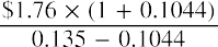


Our estimated price for this example is $63.52. Notice that the formula requires the return rate r to be greater than the growth rate g of the dividend stream. If g were greater than r, we would be dividing by a negative number and producing a negative price, which would be meaningless.
Let’s pick another company and see if we can apply the dividend growth model and price the company’s stock with a different dividend history. In addition, our earlier example will provide a shortcut method to estimate g, although you could still calculate each year’s percentage change and then average the changes over the 10 years.
Estimating a Stock Price from a Past Dividend Pattern Problem:
Phased Solutions Inc. has paid the following dividends per share from 2011 to 2020:
|
2011 |
2012 |
2013 |
2014 |
2015 |
2016 |
2017 |
2018 |
2019 |
2020 |
|
$0.070 |
$0.080 |
$0.925 |
$1.095 |
$1.275 |
$1.455 |
$1.590 |
$1.795 |
$1.930 |
$2.110 |
Table 11.4
If you plan to hold this stock for 10 years, believe Phased Solutions will continue this dividend pattern forever, and you want to earn 17% on your investment, what would you be willing to pay per share of Phased Solutions stock as of January 1, 2021?
Solution:
First, we need to estimate the annual growth rate of this dividend stream. We can use a shortcut to determine the average growth rate by using the first and last dividends in the stream and the time value of money equation. We want to find the average growth rate given an initial dividend (present value) of $0.70, the most recent dividend (future value) of $2.11, and the number of years (n) between the two dividends, or the number of dividend changes, which is 9. So, we calculate the average growth rate as follows:


Table 11.5 shows the step-by-step process of using a financial calculator to solve for the growth rate.
StepDescriptionClear calculator registerEnter number of periods (9)EnterCE/C9 NDisplay0.0000N =9.00003Enter present value or initial dividend ($0.70) as a negative 0.7 +|- PV PV = -0.7000value
Table 11.5 Calculator Steps for Solving the Growth Rate
Step45DescriptionEnter future value or the most recent dividend ($2.11)Enter a zero value for payment as a placeholder, as this factor is not used hereCompute annual growth rateEnterDisplay2.11 FVFV =2.11000 PMTPMT 0.00006CPT I/YI/Y = 13.0427
Table 11.5 Calculator Steps for Solving the Growth Rate
The calculated growth rate is 13.04%.
We can also use Excel to set up a spreadsheet similar to the one in Figure 11.10 that will calculate this growth rate.
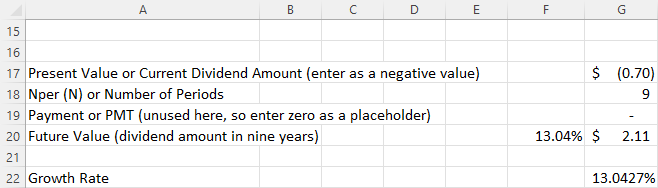
Figure 11.10 Excel Solution for Growth Rate
The Excel command used in cell G22 to calculate the growth rate is as follows:
=RATE(nper,pmt,pv,[fv],[type],[guess])
We now have two methods to estimate g, the growth rate of the dividends. The first method, calculating the change in dividend each year and then averaging these changes, is the arithmetic approach. The second method, using the first and last dividends only, is the geometric approach. The arithmetic approach is equivalent to a simple interest approach, and the geometric approach is equivalent to a compound interest approach.


To apply our PV formula above, we had to assume that the company would pay dividends forever and that we would hold on to our stock forever. If we assume that we will sell the stock at some point in the future, however, can we use this formula to estimate the value of a stock held for a finite period of time? The answer is a qualified yes. We can adjust this model for a finite horizon to estimate the present value of the dividend stream that we will receive while holding the stock. We will still have a problem estimating the stock’s selling price at the end of this finite dividend stream, and we will address this issue shortly. For the finite growing dividend stream, we adjust the infinite stream in our earlier equation to the following:
where n is the number of future dividends.
This equation may look very complicated, but just focus on the far right part of the model. This part calculates the percentage of the finite dividend stream that you will receive if you sell the stock at the end of the nth year. Say you will sell Johnson & Johnson after 10 years. What percentage of the $60.23 (the finite dividend stream) will you get? Begin with the following:


Now, multiply the result by the price for your portion of the infinite stream:


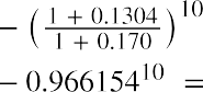
The next step is to discount the selling price of Johnson & Johnson in 10 years at 17% and then add the two values to get the stock’s price. So, how do we estimate the stock’s price at the end of 10 years? If we elect to sell the stock after 10 years and the company will continue to pay dividends at the same growth rate, what would a buyer be willing to pay? How could we estimate the selling price (value) of the stock at that time?
We need to estimate the dividend in 10 years and assume a growth rate and the required return of the new owner at that point in time. Let’s assume that the new owner also wants a 17% return and that the dividend growth rate will remain at 13.04%. We calculate the dividend in 10 years by taking the current growth rate plus one raised to the tenth power times the current dividend:


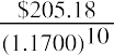
We then use the dividend growth model with infinite horizon to determine the price in 10 years as follows:
Your price for the stock today—given that you will receive the growing dividend stream for 10 years and sell for $258.10 in 10 years, and also given that you want a 17% return over the 10 years—is as shown below:


Why did you get the same price of $60.23 for your stock with both the infinite growth model and the finite model? The reason is that the required rate of return of the stock remained at 17% (your rate) and the growth rate of the dividends remained at 13.04%. The infinite growth model gives the same price as the finite model with a future selling price as long as the required return and the growth rate are the same for all future sales of the stock.
Although this point may be subtle, what we have just shown is that a stock’s price is the present value of its future dividend stream. When you sell the stock, the buyer purchases the remaining dividend stream. If that individual should sell the stock in the future, the new owner would buy the remaining dividends. That will always be the case; a stock’s buyer is always buying the future dividend stream.
LINK TO LEARNINGDetermining Stock Value Using Different ScenariosThis video explains methods for determining stock value (https://openstax.org/r/ explains_methods_for_determining_stock_value) using scenarios of constant dividends and scenarios of constant dividend growth.
THINK IT THROUGHNonconstant Growth DividendsOne final issue to address in this section is how we price a stock when dividends are neither constant nor growing at a constant rate. This can make things a bit more complicated. When a future pattern is not an annuity or the modified annuity stream of constant growth, there is no shortcut. You have to estimate every

future dividend and then discount each individual dividend back to the present. All is not lost, however. Sometimes you can see patterns in the dividends. For example, a firm might shift into a dividend stream pattern that will allow you to use one of the dividend models to take a shortcut for pricing the stock. Let’s look at an example.
JM and Company is a small start-up firm that will institute a dividend payment—a $0.25 dividend—for the first time at the end of this year. The company expects rapid growth over the next four years and will increase its dividend to $0.50, then to $1.50, and then to $3.00 before settling into a constant growth dividend pattern with dividends growing at 5% every year (see Table 11.6). If you believe that JM and Company will deliver this dividend pattern and you desire a 13% return on your investment, what price should you pay for this stock?
|
T1 |
T2 |
T3 |
T4 |
T5 |
|
|
$0.25 |
$0.50 |
$1.50 |
$1.275 |
$3.00 |
|


Table 11.6
Solution: To price this stock, we will need to discount the first four dividends at 13% and then discount the constant growth portion of the dividends, the first payment of which will be received at the end of year 5. Let’s calculate the first four dividends:
We now turn to the constant growth dividend pattern, where we can use our infinite horizon constant growth model as follows:
This figure is the price of the constant growth portion at the end of the fourth period, so we still need to discount it back to the present at the 13% required rate of return:
So, the price of this stock with a nonconstant dividend pattern is
Some Final Thoughts on Dividend Discount Models
The dividend used to calculate a price is the expected future payout and expected future dividend growth. This means the DDM is most useful when valuing companies that have long, consistent dividend records.
If the DDM formula is applied to a company with a limited dividend history, or in an industry exposed to significant risks that could affect a company’s ability to maintain its payout, the resulting derived value may not be entirely accurate.
In most cases, dividend models, whether constant growth or constant dividend, appeal to a fundamental concept of asset pricing: the future cash flow to which the owner is entitled while holding the asset and the required rate of return for that cash flow determine the value of a financial asset. However, problems can arise when using these models because the timing and amounts of future cash flows may be difficult to predict.
11.3
Discounted Cash Flow (DCF) Model
Learning Outcomes
By the end of this section, you will be able to:
- Explain how the DCF model differs from DDMs.
- Apply the DCF model.
- Explain the advantages and disadvantages of the DCF model.
When investors buy stock, they do so in order to receive cash inflows at different points in time in the future. These inflows come in the form of cash dividends (provided the stock does indeed pay dividends, because not all do) and also in the form of the final cash inflow that will occur when the investor decides to sell the stock.
The investor hopes that the final sale price of the stock will be higher than the purchase price, resulting in a capital gain. The hope for capital gains is even stronger in the case of stocks that do not pay dividends. When securities have been held for at least one year, the seller is eligible for long-term capital gains tax rates, which are lower than short-term rates for most investors. This makes non-dividend-paying stocks even more attractive, provided that they do indeed appreciate in value over the investor’s holding period. Meanwhile, short-term gains, or gains made on securities held for less than one year, are taxed at ordinary income tax rates, which are usually higher and offer no particular advantage to an investor in terms of reducing their taxes.
Understanding How the DCF Model Differs from DDMs
The valuation of an asset is typically based on the present value of future cash flows that are generated by the asset. It is no different with common stock, which brings us to another form of stock valuation: the discounted cash flow (DCF) model. The DCF model is usually used to evaluate firms that are relatively young and do not pay dividends to their shareholders. Examples of such companies include Facebook, Amazon, Google, Biogen, and Monster Beverage. The DCF model differs from the dividend discount models we covered earlier, as DDM methodologies are almost entirely based on a stock’s periodic dividends.
The DCF model is an absolute valuation model, meaning that it does not involve comparisons with other firms within any specific industry but instead uses objective data to evaluate a company on a stand-alone basis. The DCF model focuses on a company’s cash flows, determining the present value of the entire organization and then working this down to the share-value level based on total shares outstanding of the subject organization. This highly regarded methodology is the evaluation tool of choice for experienced financial analysts when evaluating companies and their common stock. Many analysts prefer DCF methods of valuation because these are based on a company’s cash flows, which are far less easily manipulated through accounting treatments than revenues or bottom-line earnings.


 The DCF model formula in its mathematical form is presented below:


where CF1 is the estimated cash flow in year 1, CF2 is the estimated cash flow in year 2, and so on; TCF is the terminal cash flow, or expected cash flow from the ending asset sale; r is the discount rate or required rate of return; g is the anticipated growth rate of the cash flow; and n is the number of years covered in the model.
Applying the DCF Model
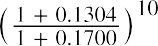
We can apply the DCF model to an example to demonstrate this methodology and how the formula works. Calculate the value of Mayweather Inc. and its common stock based on the next six years of cash flow results. Assume that the discount rate (required rate of return) is 8%, Mayweather’s growth rate is 3%, and the terminal value (TCF) will be two and one-half times the discounted value of the cash flow in year 6.
Mayweather has a cash flow of $2.0 million in year 1, so its discounted cash flow after one year (CF1) is
$1,851,851.85. We arrive at this amount by applying the discount rate of 8% for a one-year period to determine the present value.
In subsequent years, Mayweather’s cash flow will be increasing by 3%. These future cash flows also must be discounted back to present values at an 8% rate, so the discounted cash flow amounts over the next six years will be as follows:
Year 1: $1,851,852
Year 2: $1,766,118
Year 3: $1,684,353
Year 4: $1,606,374
Year 5: $1,532,005
Year 6: $1,461,079


 Our earlier assumption that the terminal value will be 2.5 times the value in the sixth year gives us a total terminal cash flow (TCF) of, or $3,652,697. Now, if we take all these future discounted cash flows and add them together, we arrive at a grand total of $13,554,477. So, based on our DCF model analysis, the total value of Mayweather Inc. is just over $13.5 million.
At this point, we have the estimated value of the entire company, but we need to work this down to the level of per-share value of common stock.


Let’s say that Mayweather is currently trading at $12 per share, and it has 1,000,000 common shares outstanding. This tells us that the market capitalization of the company is, or $12 million, and that a $12 share price may be considered relatively low. The reason for this is that based on our DCF model analysis, investors would theoretically be willing to pay $13,554,477 divided by 1,000,000 shares, or
$13.55 per share, for Mayweather. The overall conclusion would be that at $12.00 per share, Mayweather common stock would be a good buy at the present time. Figure 11.11 shows the Excel spreadsheet approach for arriving at the total value of Mayweather.
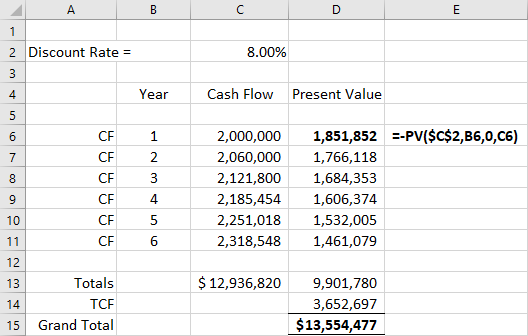
Figure 11.11 Excel Solution for Total Value
Cell E6 displays the present value formula that is active in cell D6.
Advantages and Limitations of the DCF Model
Due to several corporate accounting scandals in recent years, many analysts have given increasing credence to the use of cash flow as a metric for determining accurate corporate valuations. However, it should be noted that cash flow is not always the best means of measuring financial health. A company can always sell a large portion of its assets to generate a positive cash flow, even if it is operating at a loss or experiencing other financial difficulties. Additionally, investors prefer to see companies reinvesting their cash back into their businesses rather than sitting on excessive balances of idle cash.
Similar to other models, the discounted cash flow model is only as good as the information entered. As the common expression goes, “garbage in, garbage out.” This can often be the case if reasonably accurate cash flow estimates are not available or if an unrealistic discount rate or required rate of return is used in the calculations. It is always best to use several different methods when valuing companies and their common stock.
LINK TO LEARNINGDiscounted Cash FlowPlease view this short video on discounted cash flow (https://openstax.org/r/short_video_on_discounted) and how this method can be applied in stock valuation.
11.4
Preferred Stock
Learning Outcomes
By the end of this section, you will be able to:
- Define preferred stock.
- Calculate the intrinsic value of preferred stock.
- Understand the difference between common stock and preferred stock.
Features of Preferred Stock
Preferred stock is a unique form of equity sold by some firms that offers preferential claims in ownership. Preferred stock will often feature a dividend that a company is obligated to pay out before it makes any dividend payments to common stockholders. In cases of bankruptcy and liquidation of the issuing company, preferred stockholders have priority claim to assets before common stockholders. Additionally, preferred stockholders are usually entitled to a set (or constant) dividend every period.
Preferred stock carries a stated par value, but unlike bonds, they have no maturity date, and consequently, there is no final payment of the par value. The only time a company would pay this par value to the shareholder would be if the company ceased operations or retired the preferred stock. Many preferred stock issues are cumulative in nature, meaning that if a company skips or is otherwise unable to pay a cash dividend, it becomes a liability to the company and must eventually be paid out to preferred shareholders at some point in the future. Other preferred stocks may be noncumulative, in which case if the company skips dividends, they are forever lost to the shareholder.
The term preferred comes from preferred shareholders receiving all past (if cumulative) and present dividends before common shareholders receive any cash dividends. In other words, preferred shareholders’ dividend claims are given preferential treatment over those of common shareholders. Preferred stock is usually a form of permanent funding, but there are circumstances or covenants that could alter the payoff stream.
For example, a company may convert preferred stock into common stock at a preset point in the future. It is not uncommon for companies to issue preferred stock that has a conversion feature. Such conversion features give preferred shareholders the right to convert to common shares after a predetermined period.
A review of the characteristics of preferred stock will lead to the conclusion that the constant growth dividend model is an excellent approach for valuing such stock. Because shares of preferred stock provide a constant cash dividend based on original par value and the stated dividend rate, these may be considered a form of perpetuity.
It is this constant, preferred dividend stream that makes preferred stock seem more like bonds or another form of debt than like stock. In addition, the constant dividend stream leads nicely to the pricing of preferred stock with the four dividend models we presented earlier in this chapter.
Determining the Intrinsic Value of Preferred Stock
We can apply a version of the present value of a perpetuity formula to value preferred stock, as in the following example. Oh-Well Heath Services Inc. has issued preferred stock that has a par value of $1,000 and pays an annual dividend rate of 5%. If the market considers the risk of Oh-Well to warrant a 10% discount rate, what would be a fair market price for Oh-Well preferred stock?

 First, we find the dividend value of Oh-Well:


We then use the constant dividend model with infinite horizon because we have g equal to zero and n equal to infinity:

We can also rearrange the formula to determine the required return on this stock, given its annual dividend and current price.
 THINK IT THROUGHCalculating the Return on Preferred StockData Forge Inc. has just issued preferred stock (cumulative) with a par value of $100.00 and an annual dividend rate of 7%. The preferred stock is currently selling for $35.00 per share. What is the yield or return on this preferred stock?Solution:The first step is to determine the annual dividend by multiplying the dividend rate by the par value:Now, using this $7.00 annual dividend, the $35.00 current price, and the equation above, we calculate the rate of return as follows:
We have introduced the concept of return here, which should be thought of as both the anticipated return for the preferred stockholder and the company’s cost of borrowing money for this particular type of capital.
Differences between Preferred and Common Stock
As we have discussed, preferred stock has important differences from common stock that apply to issuing firms and to investors. Some of the most important of these differences are listed in Table 11.7.
FeatureCommon StockPaid only after preferred stockholders are paidVariable and may increase or decreaseHigh potential but tied to company performancePreferred StockDividendsHighest priority, paid firstDividendsPredetermined rates, so constant dividend amountsGrowthLiquidation Paid out last, after all creditors andpreferred stockholders are paidGiven preference in terms of payments, similar tobondsVotingRightsYesNoArrearsNo accrual of missed dividendsCertaintyDividends potentially not paid if company earns no profitsIf cumulative, unpaid dividends become liability that must be paid out eventuallyDividends paid even when company experiences financial losses
Table 11.7 Differences between Common Stock and Preferred Stock
11.5
Efficient Markets
Learning Outcomes
By the end of this section, you will be able to:
- Understand what is meant by the term efficient markets.
- Understand the term operational efficiency when referring to markets.
- Understand the term informational efficiency when referring to markets.
- Distinguish between strong, semi-strong, and weak levels of efficiency in markets.
Efficient Markets
For the public, the real concern when buying and selling of stock through the stock market is the question, “How do I know if I’m getting the best available price for my transaction?” We might ask an even broader question: Do these markets provide the best prices and the quickest possible execution of a trade? In other words, we want to know whether markets are efficient. By efficient markets, we mean markets in which costs are minimal and prices are current and fair to all traders. To answer our questions, we will look at two forms of efficiency: operational efficiency and informational efficiency.
Operational Efficiency
Operational efficiency concerns the speed and accuracy of processing a buy or sell order at the best available price. Through the years, the competitive nature of the market has promoted operational efficiency.
In the past, the NYSE (New York Stock Exchange) used a designated-order turnaround computer system known as SuperDOT to manage orders. SuperDOT was designed to match buyers and sellers and execute trades with confirmation to both parties in a matter of seconds, giving both buyers and sellers the best
available prices. SuperDOT was replaced by a system known as the Super Display Book (SDBK) in 2009 and subsequently replaced by the Universal Trading Platform in 2012.
NASDAQ used a process referred to as the small-order execution system (SOES) to process orders. The practice for registered dealers had been for SOES to publicly display all limit orders (orders awaiting execution at specified price), the best dealer quotes, and the best customer limit order sizes. The SOES system has now been largely phased out with the emergence of all-electronic trading that increased transaction speed at ever higher trading volumes.
Public access to the best available prices promotes operational efficiency. This speed in matching buyers and sellers at the best available price is strong evidence that the stock markets are operationally efficient.
Informational Efficiency
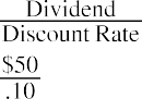
A second measure of efficiency is informational efficiency, or how quickly a source reflects comprehensive information in the available trading prices. A price is efficient if the market has used all available information to set it, which implies that stocks always trade at their fair value (see Figure 11.12). If an investor does not receive the most current information, the prices are “stale”; therefore, they are at a trading disadvantage.
Figure 11.12 Forms of Market Efficiency A market is efficient if it provides all information that is available.
Forms of Market Efficiency
Financial economists have devised three forms of market efficiency from an information perspective: weak form, semi-strong form, and strong form. These three forms constitute the efficient market hypothesis.
Believers in these three forms of efficient markets maintain, in varying degrees, that it is pointless to search for undervalued stocks, sell stocks at inflated prices, or predict market trends.
In weak form efficient markets, current prices reflect the stock’s price history and trading volume. It is useless to chart historical stock prices to predict future stock prices such that you can identify mispriced stocks and routinely outperform the market. In other words, technical analysis cannot beat the market. The market itself is the best technical analyst out there.
 Summary
Multiple Approaches to Stock Valuation
This section introduced common stock and some of the models and calculation methods used by investors and financial analysts to determine the prices or values of common shares. The most evaluative ratios that can be computed from a company’s financial statements include the price-to-earnings (P/E), price-to book (P/B), price-to-sales (P/S), and price-to cash-flow (P/CF) ratios.
Dividend Discount Models (DDMs)
The dividend discount model, or DDM, is a method used to value a stock based on the concept that its worth is the present value of all of its future dividends. The most common DDM is the Gordon growth model, which values stock entirely on expected future dividends. Other techniques include the zero growth DDM, which depends on fixed dividends; the constant growth DDM, which assumes that dividends will grow at a constant rate; and the variable growth or nonconstant growth DDM, which is based on the assumption that stock value will progress through different stages of growth. There is also the two-stage DDM, which is based on the assumption of two stages of dividend growth: an initial period of higher growth and a subsequent period of lower, more stable growth.
Discounted Cash Flow (DCF) Model
Investors buy stock to receive cash inflows at different points in the future. These inflows may come in the form of dividends or a final cash inflow. If the investor chooses to wait for a final cash flow, the hope is that capital gains will be even stronger. The DCF model is usually used to evaluate firms that are relatively young and do not pay dividends to their shareholders. The DCF model focuses on a company’s cash flows, determining the present value of an entire organization using objective data and then working this down to the share-value level based on total shares outstanding of the subject organization.
Preferred Stock
Preferred stock is a unique form of equity sold by some firms that offers preferential claims in ownership. Preferred stock carries a stated par value, but unlike bonds, there is no maturity date, and consequently, there is no final payment of the par value. The term preferred comes from preferred shareholders receiving all past (if cumulative) and present dividends before common shareholders receive any cash dividends.
Efficient Markets
Efficient markets are markets in which costs are minimal and prices are current and fair to all traders. There are two forms of efficiency: operational efficiency and informational efficiency. Operational efficiency concerns the speed and accuracy of processing a buy or sell order at the best available price. Informational efficiency concerns how quickly a source reflects comprehensive information in the available trading prices. Financial economists have devised three forms of efficient markets from an information perspective: weak form, semi- strong form, and strong form.
 Key Terms
amortization the process of spreading business costs in accounting; similar to depreciation, but differs in that it generally refers to intangible assets such as patents or copyrights
capital employed also known as funds employed; the total amount of capital used for the acquisition of profits by a firm or on a project
common stock a security that represents partial ownership of a corporation
comparable company analysis (comps) a method for valuating a company using the metrics of other businesses of similar size in the same industry
depreciation the process of spreading business costs in accounting; similar to amortization, but differs in
that it generally refers to fixed, tangible assets such as buildings, machinery, furniture, fixtures, and equipment
discounted cash flow (DCF) a method for estimating the value of an investment based on the present value of its expected future cash flows
dividend a sum of money paid regularly (typically quarterly) by a company to its shareholders out of its profits or reserves
dividend discount model (DDM) a quantitative method for predicting the price of a company’s stock based on the theory that its present-day price is worth the sum of all of its future dividend payments when discounted back to their present value
dividend yield a financial ratio (dividend/price) that shows how much a company pays out in dividends each year relative to its stock price, expressed as a percentage
earnings per share (EPS) the ratio of a company’s profits to the outstanding shares of its common stock; serves as an indicator of a company’s profitability
EBIT short for earnings before interest and taxes; an indicator of a firm’s profitability before the effects of interest or taxes; also referred to as operating earnings, operating profit, and profit before interest and tax
efficient markets markets in which costs are minimal and prices are current, fair, and reflective of all available relevant information
enterprise value (EV) a company’s total value; often used as a more comprehensive alternative to equity market capitalization
enterprise value (EV) multiples also known as company value multiples; ratios used to determine the overall value of a company and, by extension, the value of its common stock
equity multiples metrics that calculate the expected or achieved total return on an initial investment
Gordon growth model a methodology used to determine the intrinsic value of a stock based on a future series of dividends that grow at a constant rate
growth rate the rate at which the dollar amount of dividends paid on a specific stock holding increases
intangible assets assets that are not physical in nature, such as goodwill, brand recognition, and intellectual property (i.e., patents, trademarks, and copyrights)
intrinsic value the value of a firm’s stock based entirely on internal factors, such as products, management, and the strength of company brands in the marketplace
market capitalization the value of a company traded on the stock market, calculated by multiplying the total number of shares by the current share price
NASDAQ (National Association of Securities Dealers Automated Quotations) short for National Association of Securities Dealers Automated Quotations; an American stock exchange based in New York City, ranked second behind the New York Stock Exchange in terms of total market capitalization of shares traded
net book value also called net asset value (NAV); the total assets of a company minus its total liabilities
NYSE (New York Stock Exchange) the world’s largest stock exchange by market capitalization of its listed companies, based in New York City; often referred to as the “Big Board”
perpetuity in terms of investments, an annuity with no end date
precedent transaction analysis (precedents) a method for valuating a company in which the price paid for similar companies in the past is considered an indicator of the company’s current value
preferred stock stock that entitles the holder to a fixed dividend, the payment of which takes priority over payment of common stock dividends
price-to-book (P/B) ratio also called the market-to-book (M/B) ratio; a metric used to compare a company’s market capitalization, or market value, to its book value
price-to-cash-flow (P/CF) ratio a stock valuation indicator or multiple that measures the value of a stock’s price relative to its operating cash flow per share
price-to-earnings (P/E) ratio a ratio that indicates the dollar amount an investor can expect to invest in a company in order to receive one dollar of that company’s earnings
price-to-sales (P/S) ratio a ratio that indicates how much investors are willing to pay for a company’s stock
per dollar of that company’s sales
required return the minimum return an investor expects to achieve by investing in a project
secondary markets markets where investors buy and sell securities they already own
stock value also called intrinsic value; the fundamental, objective value of a share of stock