8 Lesson 4c Uneven Flows

Baseball legend Ted Williams once said, “Baseball is the only field of endeavor where a man can succeed three times out of ten and be considered a good performer.”¹ On routine or unimportant decisions, business managers might aspire to do as well as Ted Williams, making the right decisions only 30% of the time. But a professional decision maker must “hit it out of the park” when making major capital investment choices and recommendations.

As a student in a course of business studies and career development, it is highly likely that you will be a decision maker about projects that are likely to generate future cash flows but will also require a large initial expense. When you ask your manager to invest $500,000 or more in a new piece of equipment that could help your department meet or exceed its goals, you must be prepared to defend your request. Competing managers and departments will be asking for similar funding, and there simply might not be enough for everyone. This decision process requires financial analysis.

Mark Cuban of Shark Tank fame enjoys citing the series’ catchphrase: “Know thy numbers.” As a business professional, you must be able to assess potential profit against expenditures to be successful. In most cases, this is based on our understanding of cash flow. A major capital investment might seem initially like a gamble, but it is a gamble that can be hedged in your favor with understanding, analysis, and knowledge of your numbers.

The purpose of this chapter is to give you information and instruction on how this is done. The techniques we will discuss in this chapter will clarify decisions that must be made in the process of investing in a business. We

• Pete Palmer and Gary Gillette, eds. The 2006 ESPN Baseball Encyclopedia. New York: Sterling Publishing, 2006, 5.

focus first on decisions we make about our own money as investors if uneven cash receipts or payments are involved.

9.1
Timing of Cash Flows

Learning Outcomes

By the end of this section, you will be able to:

• Describe how multiple payments of unequal value are present in everyday situations.
• Calculate the future value of a series of multiple payments of unequal value.
• Calculate the present value of a series of multiple payments of unequal value.

Multiple Payments or Receipts of Unequal Value: The Mixed Stream

At this point, you are familiar with the time value of money of single amounts and annuities and how they must be managed and controlled for business as well as personal purposes. If a stream of payments occurs in which the amount of the payments changes at any point, the techniques for solving for annuities must be modified. Shortcuts that we have seen in earlier chapters cannot be taken. Fortunately, with tools such as financial or online calculators and Microsoft Excel, the method can be quite simple.

The ability to analyze and understand cash flow is essential. From a personal point of view, assume that you have an opportunity to invest $2,000 every year, beginning next year, to save for a down payment on the purchase of your first home seven years from now. In the third year, you also inherit $10,000 and put it all toward this goal. In the fifth year, you receive a large bonus of $3,000 and also dedicate this to your ongoing investment.

The stream of regular payments has been interrupted—which is, of course, good news for you. However, it does add a new complexity to the math involved in finding values related to time, whether compounding into the future or discounting to the present value. Analysts refer to such a series of payments as a mixed stream. If you make the first payment on the first day of next year and continue to do so on the first day of each following year, and if your investment will always be earning 7% interest, how much cash will you have accumulated—principal plus earned interest—at the end of the seven years?

This is a future value question, but because the stream of payments is mixed, we cannot use annuity formulas or approaches and the shortcuts they provide. As noted in previous chapters, when solving a problem involving the time value of money, a timeline and/or table is helpful. The cash flows described above are shown in Table 9.1 . Remember that all money is assumed to be deposited in your investment at the beginning of each year. The cumulative cash flows do not yet consider interest.

Year	0	1	2	3	4	5	6	7
Cash Invested	$0.00	$2,000	$2,000	$2,000	$12,000	$2,000	$5,000	$2,000
Cumulative Cash Flows		$2,000	$4,000	$6,000	$18,000	$20,000	$25,000	$27,000

Table 9.1

By the end of seven years, you have invested $27,000 of your own money before we consider interest:

• Seven years times $2,000 each year, or $14,000
• The extra $10,000 you received in year 3 (which is invested at the start of year 4)
• The extra $3,000 you received in year 5 (which is invested at the start of year 6)

These funds were invested at different times, and time and interest rate will work for you on all accumulated balances as you proceed. Therefore, focus on the line in your table with the cumulative cash flows. How much cash will you have accumulated at the end of this investment program if you’re earning 7% compounded

annually? You could use the future value of a single amount equation, but not for an annuity. Because the amount invested changes, you must calculate the future value of each amount invested and add them together for your result.

Recall that the formula for finding the future value of a single amount is, where FV is the future value we are trying to determine, PV is the value invested at the start of each period, i is the interest rate, and n is the number of periods remaining for compounding to take effect.

Let us repeat the table with your cash flows above. Table 9.2 includes a line to show for how many periods (years, in this case) each investment will compound at 7%.

Year	0	1	2	3	4	5	6	7
Cash Invested	$0.00	$2,000	$2,000	$2,000	$12,000	$2,000	$5,000	$2,000
Cumulative Cash Flows		$2,000	$4,000	$6,000	$18,000	$20,000	$25,000	$27,000
Years to Compound		7	6	5	4	3	2	1

Table 9.2

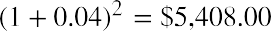
The $2,000 that you deposit at the start of year 1 will earn 7% interest for the entire seven years. When you make your second investment at the start of year 2, you will now have spent $4,000. However, the interest from your first $2,000 investment will have earned you , so you will begin year 2 with

$4,140 rather than $4,000.

Before we complicate the problem with a schedule that ties everything together, let’s focus on years 1 and 2 with the original formula for the future value of a single amount. What will your year 1 investment be worth at the end of seven years?

You need to address the year 2 investment separately at this point because you’ve calculated the year 1 investment and its compounding on its own. Now you need to know what your year 2 investment will be worth in the future, but it will only compound for six years. What will it be worth?

You can perform the same operation on each of the remaining five invested amounts, remembering that you invest $12,000 at the start of year 4 and $5,000 at the start of year 6, as per the table. Here are the five remaining calculations:

Notice how the exponent representing n decreases each year to reflect the decreasing number of years that each invested amount will compound until the end of your seven-year stream. For clarity, let us insert each of these amounts in a row of Table 9.3 :

Year	0	1	2	3	4	5	6	7
Cash Invested	$0.00	$2,000	$2,000	$2,000	$12,000	$2,000	$5,000	$2,000
Cumulative Cash Flows		$2,000	$4,000	$6,000	$18,000	$20,000	$25,000	$27,000

Table 9.3

Year	0	1	2	3	4	5	6	7
Years to Compound		7	6	5	4	3	2	1
Compounded Value at End of Year 7		$3,211.56	$3,001.46	$2,805.10	$15,729.55	$2,450.09	$5,724.50	$2,140.00

Table 9.3

The solution to the original question—the value of your seven different investments at the end of the seven- year period—is the total of each individual investment compounded over the remaining years. Adding the compounded values in the bottom row provides the answer: $35,062.26. This includes the $27,000 that you invested plus $8,062.26 in interest earned by compounding.

It’s important to note that throughout these sections on the time value of money and compounded or discounted values of mixed streams and their analysis, we are placing the valuation at the end or beginning of a period for simplicity in the examples. In reality, businesses might consider valuations happening within the period to allow for a degree of regularity in the revenue streams provided by the asset being considered.

THINK IT THROUGHFuture Value of a Mixed StreamAssume that you can invest five annual payments of $10,000, beginning immediately, but you believe you will be able to invest additional amounts of $5,000 at the beginning of years 4 and 5. This investment is expected to earn 4% each year. What is the anticipated future value of this investment after the full five years?Solution:Table 9.4The equations to calculate each individual year’s compounded value at the end of the five years are asfollows:The sum of these individual calculations is $66,937.76, which is the total value of this stream of investedamounts plus compounded interest.
However, because this is a technique of forecasting, which is inherently uncertain, we will continue with analysis by period.

Year	0	1	2	3	4	5
Cash Invested	$0.00	$10,000	$10,000	$10,000	$15,000	$15,000
Cumulative Cash Flows		$10,000	$20,000	$30,000	$45,000	$60,000
Years to Compound		5	4	3	2	1
Compounded Value at End of Year 5		$12,166.53	$11,698.59	$11,248.64	$16,224.00	$15,600.00

Let’s take the example above and review it from a different angle. Keeping in mind that we have not yet explored the use of Excel, is there another way to view our solution? The problem above takes each annual investment and compounds it into the future, then adds the results of each calculation to find the total future value of the stream of payments.

But when you break the problem down, another way to look at the problem is as a five-year annuity of $10,000 per year plus added payments in years 4 and 5. Can we solve for the future value of an annuity first and then perform two separate calculations on the additional amounts ($5,000 each in years 4 and 5)? Yes, we can.

Let’s summarize:

• Future value of a $10,000 annuity due, 4%, 5 years, plus
• Future value of a single payment of $5,000, 4%, 2 years, plus
• Future value of a single payment of $5,000, 4%, 1 year

This must give us the same result. The formula for the future value of an annuity due is

This problem can be solved in the three steps of the summary above. Step 1:

Step 2:

Step 3:

Combining the results from each of the three steps gives us

It works. Whether you view this problem as five separate periods that can be compounded separately and then combined or as a combination of one or more annuities and/or single payment problems, we always arrive at the same solution if we are diligent about the time, the interest, and the stream of payments.

The Present Value of a Mixed Stream

Now that we’ve seen the calculation of a future value, consider a present value. We will begin with a personal example. You win a cash windfall through your state’s lottery. You would like to take a portion of the funds and place them in a fixed investment so that you can draw $17,000 per year starting one year from now and continue to do so for the next two years. At the end of year 4, you want to withdraw $17,500, and at the end of year 5, you will withdraw the last $18,000 to close the account. When you take your last payment of

$18,000, your fund will be totally depleted. You will always be earning 6% annually. How much of your cash windfall should you set aside today to accomplish this?

Let us break down the problem, remembering that we are thinking in reverse from the earlier problems that involved future values. In this case, we’re bringing future values back in time to find their present values. You will recall that this process is called discounting rather than compounding.

Regardless of how we solve this, the question remains the same: How much money must we invest today (present value) to achieve this? And remember that we will always be earning 6% compounded annually on any invested balances.

We are calculating present values as we did in previous chapters, given a known future value “target,” in order to determine how much money you need today to achieve that goal. Let us break this down by first reviewing the relevant equations from previous chapters.

Present value of an ordinary annuity:

Present value of a single amount:

where PVa is the present value of an annuity, PYMT is one payment in a consistent stream (an annuity), i is the interest rate (annual unless otherwise specified), n is the number of periods, PV is the present value of a single amount, and FV is the future value of a single amount.

You want to find out how much money you need to set aside today to accomplish your goal. You can also find out how much money you need to set aside in each period to accomplish this goal. Therefore, we can address this problem in increments. Let us look at potential solutions.

First, we will break this down into the cash flows of each year. Table 9.5 shows the timing of the future cash flows you’re expecting:

Year	0	1	2	3	4	5
Expected Amount to Be Withdrawn at End of Year	$0.00	$17,000	$17,000	$17,000	$17,500	$18,000

Table 9.5

One method is to take each year’s cash flows, which happen at the end of the year, and discount them to today using the present value formula for a single amount:

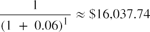
Because year 1’s withdrawal from your fund only has one year to earn interest, we discounted it for one year. The second amount is discounted for two years:

The next three years are discounted in the same way, for three, four, and five years, respectively:

Notice how we reverse our thinking on the exponent n from our approach to future value. This time, it increases each period because we discount each future amount for a longer period to arrive at the value in today’s dollars.

When we add all five discounted present value amounts from above, we derive today’s value of $72,753.49. Expressed more simply, if you wanted to extract the specified stream of cash flows at the end of each year

($17,000 for three years, then $17,500, then $18,000), you would have to begin with $72,753.49. The thing to remember is that any amounts remaining in this fund, regardless of how you deplete it, will always be earning 6% annually. See Table 9.6.

Year	0	1	2	3	4	5
Withdrawn at End of Year		$17,000.00	$17,000.00	$17,000.00	$17,500.00	$18,000.00
Interest on Balance		$4,365.21	$3,607.12	$2,803.55	$1,951.76	$1,018.87
Remaining Balance	$72,753.49	$60,118.70	$46,725.82	$32,529.37	$16,981.13	$0.00

Table 9.6

Let us try another approach. Because the amount of cash withdrawn in the first three years remains constant at $17,000, it can be viewed as an annuity—specifically, a three-period annuity of $17,000 and two single payments of $17,500 and $18,000. Therefore, we could also discount (bring to present value) an annuity of

$17,000 for three years (the first three) and then combine it with the year 4 discounted amount and the year 5 discounted amount. We can try it using the formulas for PVa and PVused above. In Step 1, we will discount the first three years as an annuity (ordinary, as the first withdrawal is not made until one year from now); in Step 2, we will discount the year 4 single payment amount; and in Step 3, we will do the same for the year 5 single payment amount. Then we can add them together.

Step 1: Find the present value of the annuity using the PVa formula:

Step 2: Discount the year 4 amount using the formula for the present value of a single amount:

Step 3: Perform the same operation as in Step 2 for the year 5 amount:

Now that all three amounts have been discounted to today’s value, we can add them:

Calculating the present value of cash flows is very common and critical in the analysis of capital investments in business for two compelling reasons: first, the investment is likely quite significant, and second, the risk will usually encompass a longer time frame. When the author of this chapter would purchase a large machine, it would likely take several years for that machine to justify its purchase with the revenues it would generate.

This is one of the primary reasons that accountants require us to depreciate the cost of an asset over time: to assess the cost against the time it will take for that asset to produce profits and cash flow.

THINK IT THROUGH

Present Value of a Mixed Stream

Assume that you decide to invest $450,000. All cash flows are discounted at 4%. You are told by your financial advisor to expect cash inflows from your investment of $100,000 in year 1, $125,000 in year 2,

$175,000 in year 3, $90,000 in year 4, and $50,000 in year 5. Would you agree to this plan based only on the numbers? Each amount will be withdrawn at the end of every year, and interest will be compounded annually.

Solution:

Year	0	1	2	3	4	5
Expected Amount to Be Withdrawn at End of Year	$0.00	$100,000	$125,000	$175,000	$90,000	$50,000

Table 9.7

Applying the formula for the present value of a single amount, we discount each amount and then add the discounted amounts. We will simplify this approach with Excel shortly, but we must understand the reasoning behind discounting uneven cash flow streams with a direct solution.

By combining the five discounted amounts above, we get a total present value of $485,326.48. This amount represents the value today of the five expected cash inflows for as long as our remaining balance is earning 4%.

CONCEPTS IN PRACTICEThoughts on Cash Flow from Irina SimmonsIn 2013, the author interviewed Irina Simmons, senior vice president, chief risk officer, and former treasurer of EMC Corporation. The importance and understanding of cash flow analysis is fundamental to this text, and several of her insights are highly relevant to our content and procedures here.AA: Ms. Simmons, why is cash management so important to an existing or start-up firm, and how does it compare to the more basic and traditional focus on profitability?Simmons: While profitability is very useful for analysis by investors to measure performance, an organization’s cash flow provides superior measurement. Cash flow is easy to understand, provides a transparent way of assessing a firm’s health, and is not subject to any qualifications. By focusing upon cash flow, any firm—whether it is mature or a start-up organization—can have a clear picture of its health and success.

AA: In your bio, you mention liquidity management. Can you elaborate on this and why liquidity management is so important to a firm?

Simmons: Just as effective forecasting can provide superior cash management, the same holds true for liquidity management. For example, if you are able to confidently predict levels and timing of cash, then based on that forecast, you can make effective short- and long-term borrowing decisions. A disciplined approach to projecting one’s cash position means that instead of investing cash in the money market to maximize day-to-day liquidity, you can look into longer-term investments that can provide a significantly higher return. This is essential to the effective matching of cash inflows and outflows for the firm.

AA: In summary, do you have any words of advice to students who might have an eye to entrepreneurial ventures?

Simmons: “Cash is king,” don’t forget that. Understand how cash moves through a business. It is also very important to implement and retain a cash management discipline. Never put that off until later. Many times, start-ups will say, “Well, I have all this venture money, and we can start making things happen and worry about being good cash managers later.” But what I’ve seen is that the longer companies wait, the harder it is to break bad habits. Making cash management a priority now will serve entrepreneurs in perfect stead as their business starts to gain traction.

We closed this excellent interview with agreement that we were “kindred spirits” regarding the importance of cash flow analysis, including capital decisions such as those mentioned in this chapter. We confirmed with each other the core belief that “cash flow is the axis upon which the world of business spins.”

(source: Business Finance: A Clear View, 3rd edition, by Alan S. Adams. LAD Publishing, 2015.)

LINK TO LEARNINGAnalyst Training MaterialsThese materials, developed to help professionals prepare for an analyst certification exam, describe the sources of return from investing in a bond (https://openstax.org/r/return-investing-bond).

9.2
Unequal Payments Using a Financial Calculator or Microsoft Excel

Learning Outcomes

By the end of this section, you will be able to:

• Calculate unequal payments using a financial calculator.
• Calculate unequal payments using Microsoft Excel.

Using a Financial Calculator

A financial calculator provides utilities to simplify the analysis of uneven mixed cash streams (see Table 9.8).

Earlier, we explored the future value of a seven-year mixed stream, with $2,000 being saved each year, plus an additional $10,000 in year 4 and an additional $3,000 in year 6. All cash flows and balances earn 7% per year compounded annually, and the payments are made at the start of each year. We proved that this result totals approximately $35,062.26. We begin by clearing all memory functions and then entering each cash flow as follows:

Step1234567891011121314151617181920DescriptionClear cash flow memoryEnter 0 for cash flow at Time 0 Move to next entryEnter first cash flow Move to next entry Enter second cash flow Move to next entry Enter third cash flow Move to next entry Enter fourth cash flow Move to next entry Enter fifth cash flow Move to next entry Enter sixth cash flow Move to next entry Enter seventh cash flow Press NPVEnter interest rateEnterCF 2ND [CLR WORK] CF0ENTER ↓↓2000 ENTER↓ ↓2000 ENTER ↓↓ ↓2000 ENTER↓ ↓12000 ENTER↓ ↓2000 ENTER↓ ↓5000 ENTER↓ ↓2000 ENTER NPV7 ENTERCF0C01Display0.000.000.00C01 = C02 C02 = C03 C03 =C042000.000.002000.000.002000.000.00C04 = 12000.00Press down arrow to show current NPV rate ↓Press CPT to find net present valueCPTC05 C05 = C06 C06 = C07 C07 = II = NPVNPV0.002000.000.005000.000.002000.000.007.000.0020,406.56

Table 9.8 Steps for Calculating Uneven Mixed Cash Flows²

At this point, we have found the net present value of this uneven stream of payments. You will recall, however, that we are not trying to calculate present values; we are looking for future values. The TI BA II Plus™ Professional calculator does not have a similar function for future value. This means that either we can find the future value for each payment in the stream and combine them, or we can take the net present value we just calculated and easily project it forward using the following keystrokes. Note the net present value solution in Step 20 above. We will use that and then use the simpler of the two approaches to calculate future value (see Table 9.9).

Step21222324DescriptionEnter NPV from Step 20EnterDisplay20406.56 PV =Enter number of compounding periods 8 NEnter interest rateCalculate future value7 I/YCPT FVN =I/Y =20,406.568.007.00FV = -35,062.27

Table 9.9 Steps for Calculating Uneven Mixed Cash Flows, Continued

• The specific financial calculator in these examples is the Texas Instruments BA II PlusTM Professional model, but you can use other financial calculators for these types of calculations.

This is consistent with the solution we found earlier, with a difference of one cent due to rounding error.

We may also use the calculator to solve for the present value of a mixed cash stream. Earlier in this chapter, we asked how much money you would need today to fund the following five annual withdrawals, with each withdrawal made at the end of the year, beginning one year from now, and all remaining money earning 6% compounded annually:

Year	1	2	3	4	5
	$17,000	$17,000	$17,000	$17,500	$18,000

Table 9.10

We determined these withdrawals to have a total present value of $72,753.30. Here is an approach to a solution using a financial calculator. In this example, we will store all cash flows in the calculator and perform an operation on them as a whole (see Table 9.11). Because we will use the NPV function (to be explored in more detail in a later chapter), we enter our starting point as 0 because we do not withdraw any cash until one year after we begin.

Step12345678910111213141516DescriptionClear cash flow memoryEnter 0 for cash flow at Time 0 Move to next entryEnter first cash flow Move to next entry Enter second cash flow Move to next entry Enter third cash flow Move to next entry Enter fourth cash flow Move to next entry Enter fifth cash flow Press NPVEnter interest rateEnterDisplayCF 2ND [CLR WORK] CF0ENTER ↓↓17000 ENTER↓ ↓17000 ENTER↓ ↓17000 ENTER↓ ↓17500 ENTER↓ ↓18000 ENTER NPV6 ENTERPress down arrow to show current NPV rate ↓CF0 C01 C01 = C02 C02 = C03 C03 = C04 C04 = C05 C05 = II =NPV0.000.000.0017000.000.0017000.000.0017000.000.0017500.000.0018000.000.0060.00Press CPT to find net present valueCPTNPV = 72,753.49

Table 9.11 Steps for Calculating the Present Value of a Mixed Cash Stream

This result, you will remember, was calculated earlier in the chapter by the formula approach.

Using Microsoft Excel

Several of the exhibits already in this chapter have been prepared with Microsoft Excel. While full mastery of Excel requires extensive study and practice, enough basics can be learned in two or three hours to provide the user with the ability to quickly and conveniently solve problems, including extensive financial applications.

Potential employers and internship hosts have come to expect basic Excel knowledge, something to which you

are exposed in college.

We will demonstrate the same two problems using Excel rather than a calculator:

• The future value of a mixed cash stream for a seven-year investment
• The present value of a mixed cash stream of five withdrawals that you wish to make from a fund to be established today

Beginning with the future value problem, we created a simple matrix to lay out the mixed stream of future cash flows, starting on the first day of each year, with all funds earning 7% throughout. Our goal is to determine how much money you will have saved at the end of this seven-year period.

Table 9.12 repeats the data from earlier in the chaper for your convenience.

Year	0	1	2	3	4	5	6	7
Cash Invested	$0.00	$2,000	$2,000	$2,000	$12,000	$2,000	$5,000	$2,000
Cumulative Cash Flows		$2,000	$4,000	$6,000	$18,000	$20,000	$25,000	$27,000
Years to Compound		7	6	5	4	3	2	1

Table 9.12

Figure 9.2 is an Excel matrix that parallels Table 9.12 above.

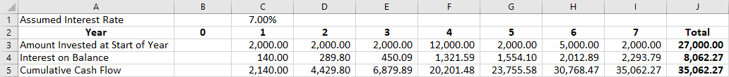
Figure 9.2 Compound Interest Example

Download the spreadsheet file (https://openstax.org/r/chapter9-excel-exhibits) containing key Chapter 9 Excel exhibits.

We begin by entering the cash flow as shown in Figure 9.2. The assumed interest rate is 7%. The interest on the balance is calculated as the amount invested at the start of the year multiplied by the assumed interest rate. The cumulative cash flows of each year are calculated as follows: for year 1, the amount invested plus the interest on the balance; for years 2 through 7, the amount invested plus the interest on the balance plus the previous year’s running balance. By adding up the amount invested and the interest on the balance, you should arrive at a total of $35,062.27.

We can use Excel formulas to solve time value of money problems. For example, if we wanted to find the present value of the amount invested at 7% over the seven-year time period, we could use the NPV function in Excel. The dialog box for this function (Rate, Value 1, Value2) is shown in Figure 9.3.

Figure 9.3 Dialog Box for NPV Function, Problem 1

The function argument Rate is the interest rate; Value1, Value2, and so on are the cash flows; and “Formula result” is the answer.

We can apply the NPV function to our problem as shown in Figure 9.4.

Figure 9.4 Applying the NPV Function, Problem 1

Please note that the Rate cell value (C1) and the Value1 cell range (C3:I3) will vary depending on how you set up your spreadsheet.

The non-Excel version of the problem, using an assumed interest rate of 7%, produces the same result.

Year	1	2	3	4	5	6	7
Amount Invested at Start	$2,000	$2,000	$2,000	$12,000	$2,000	$5,000	$2,000
NPV	$20,406.56

Table 9.13

We conclude with the second problem addressed earlier in this chapter: finding the present value of an uneven stream of payments. We can use Excel’s NPV function to solve this problem as well (see Figure 9.5).

Year	0	1	2	3	4	5
Expected Amount to Be Withdrawn at End of Year	$0.00	$17,000	$17,000	$17,000	$17,500	$18,000

Table 9.14

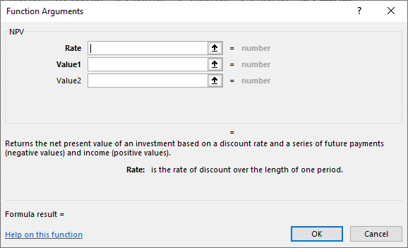
Figure 9.5 Dialog Box for NPV Function, Problem 2

Again, Rate is the interest rate; Value1, Value 2, and so on are the cash flows; and “Formula result” is the answer.

Let us apply the NPV function to our problem, as shown in Figure 9.6 and Figure 9.7.

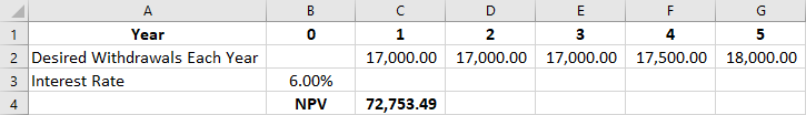
Figure 9.6 Applying the NPV Function, Problem 2: Excel Data

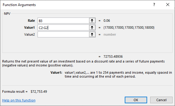
Figure 9.7 Applying the NPV Function, Problem 2: Function Argument

Please note that the Rate cell value (B3) and the Value1 cell range (C2:G2) will vary depending on how you set up your spreadsheet.

The non-Excel version of the problem produces the same result: an NPV of $72,753.49.

Year	0	1	2	3	4	5
Desired Withdrawals Each Year	$17,000	$17,000	$17,000	$17,500	$18,000
Interest Rate	0.06
NPV						$72,753.49

Table 9.15

Summary

Timing of Cash Flows

To understand the true value and strength of cash, it is necessary to consider its timing. This is relevant for investments for the future and for analyses of the value of projects that require investment today to produce expected flows of cash later. These future cash flows could involve inflows or outflows of cash in unequal amounts. This section analyzed the determination of present and future value of these uneven or mixed cash flows.

Unequal Payments Using a Financial Calculator or Microsoft Excel

This section discussed the use of two tools for managing and understanding the time value of money and its many applications when the flows of cash are unequal: the TI BA II Plus™ Professional financial calculator and the spreadsheet application Excel.

Key Terms

capital investment a major expenditure that requires a large up-front investment and is expected to generate substantial cash inflow in return

cash flow the amount of cash actually flowing into and out of a business, as opposed to income (which is based on accounting rules, accruals, and reports)

future value the value of an asset or holding at a point in the future based on expectations of that asset’s growth at a certain rate of return

mixed stream a set of cash flows over a period of time that can vary in amount from one period to the next

present value the value of an asset in today’s dollars based on future growth expectations at an assumed interest rate