7 Lesson 4 b Time Value of Money Multiple Payments

Although this text is directed at business finance students, our daily decisions as consumers are largely based on money and finance to just as great an extent. An old adage in finance claims, “If you aren’t in control of your money, your money is controlling you.” Fortunately, learning to manage your money is not difficult if you’re disciplined and understand some simple techniques. For example, several years ago, the author was negotiating for a three-year auto loan from a well-known regional dealer, who was offering an interest rate of 2%. When the manager left the room for a few minutes, we pulled out a financial calculator and proved in less than a minute that the actual interest rate in the payments he was proposing was nearly double the quoted and advertised rate.

In addition to understanding how the loan process works, which improves your negotiation skills when borrowing, businesses and individuals can better control their investments by understanding basic rules of finance, particularly as seen in this and the preceding chapter. Assume you pledge to invest $1,000 per year at 5% return per year and are curious about how much you will have accumulated by age 60. If you begin at age 30, you will have $69,760; if you begin at age 20, you will have $126,840. Can the extra 10 years make that much of a difference? We’ll see that indeed they can, and the calculations required to prove it can take less than two minutes.

As another example, many professionals confuse income and wealth during their career growth. In their popular book The Millionaire Next Door: The Surprising Secrets of America’s Wealthy, authors Thomas Stanley

and William Danko illustrate these terms with a flowing river. A river is in constant movement, and as the flow or depth increases, this is comparable to one’s income increasing through the promotions, salary increases, and bonuses one receives. Unfortunately, many individuals then increase their spending habits in response, justifying a better car, a second home, or more lavish vacations. Wealth, in contrast, is comparable to taking a bucket of water from the river and holding it aside in a tank for oneself. Financial professionals often call this “paying yourself first.” Stanley and Danko list this among the “secrets” referenced in the title of their book.

8.1
Perpetuities

Learning Outcomes

By the end of this section, you will be able to:

• Define perpetuity.
• Explain how perpetuities are valued.

In Time Value of Money I, we learned that the value of money changes with the passage of time. Decision- makers consider how investments, projects, and even opportunity costs gain value as we move forward into the future. They similarly consider how value in the future can be reduced to a value in present or past periods. We saw that these value projections are called determination of future value (compounding, moving forward on a timeline) or present value (discounting, moving backward on a timeline). The easiest way to visualize this movement through time, whether forward or backward, is by use of a timeline.

Throughout the first chapter on the time value of money, we were analyzing a single amount. In this chapter, we deal with a stream of payments made periodically—in other words, payments made or received regularly over a span of time. We begin with the illustration of a perpetuity.

What Is a Perpetuity?

A perpetuity is a series of payments or receipts that continues forever, or perpetually. One of the best ways to analyze the basics of an annuity (the stream of payments to be paid or received in the future) is by starting with a perpetuity. The most common examples of perpetuities in the author’s experience are college chair endowments and preferred stock.

If you gift $1,500,000 to a college to name a professor’s chair for your family, you might specify that the money must be held in perpetuity and invested by the college to yield a fixed 3%. The college will take those proceeds of the investment, leaving your original $1,500,000 intact, and use the annual interest of $45,000 to fund a portion of the professor’s salary.

Another common example is preferred stock. Most preferred stock issues carry a fixed and predetermined rate of dividend. If we assume that the dividend will not change in future years, then preferred dividend shareholders will receive a fixed amount of money in future years—assuming, of course, that the company’s board of directors declares the dividends sufficient to fund these requirements. If we assume that the dividend is declared and paid and that it remains constant, this represents a perpetuity.

For example, Shaw Inc. has issued 100,000 shares of preferred stock with a stated value of $50 and a 4% dividend. Therefore, if they can fund and decide to declare dividends for the full amount, they will pay out

$200,000, or $2.00 per preferred share. Because shares such as these are created with the intention of continuity, the owner of this preferred stock can theoretically expect this dividend income stream in perpetuity.

To place a current market value on this stream of future income, how much should an investor pay for one share of this preferred stock? The calculation is a present value. The amount the investor pays today for that one share is equal to the annual dividend (assuming it is declared and paid) divided by the rate of return. But be careful—it is not the rate on the face of the preferred stock but the required rate of return, the “market rate” that investors expect from a stock of this level of risk. We must also note an important fact affecting all

investment valuations: the value of an investment generally represents our expectations of all future cash flows from that investment, discounted to today’s dollars.

Because a perpetuity is a stream of payments continuing indefinitely, determining the future value isn’t possible. Determining the present value, however, is possible, although one might wonder how. As we learned earlier, the greater the amount of time used in a present value calculation, the smaller the amount of dollars needed at the beginning, regardless of the interest rate involved. Therefore, when we discount each payment in an infinite series, remembering that we would then add them together once we discount them to the present, the infinite payments become negligible at some point and will no longer have a significant impact on today’s value. To grow to one dollar 70 years from now, even at a growth rate of 5% per year, we would only need $0.0329—not even four cents. Keeping all other facts the same, if we had 100 years to grow an investment to one dollar, we would only need 0.76 cents—not even a whole penny! There is no question that the effect of time is substantial and dramatic.

The study of perpetuities in corporate finance is a first step to understanding valuation models of certain investments, such as the dividend discount model and the constant growth model, to be addressed in other chapters. Our ability to discount future cash flows, even infinite cash flows, to a present value is a clue to the price at which a company’s stock might trade. From a personal financial planning perspective, the individual investor is also better able to be certain that they are paying a fair price for holdings in their portfolio. For purposes of long-term or retirement planning, the investor must consider that a fixed and unchanging dividend, such as from preferred stock, might not adequately protect the holder from inflation in times of rising prices.

How to Value a Perpetuity

Given these facts, how do we place a value on a perpetuity? Let’s keep the preferred stock example for Shaw Inc. in mind. The holder of one share will expect to receive a $2.00 dividend for every share owned. Although a perpetuity may allow for growth of that dividend, we will hold that constant now. We must know one additional fact: the required rate of return. This is our random variable, which can cause fluctuation in the price of the preferred stock. Let’s assume that the required rate of return, which we’ll call R_S, is 7%. This is the rate of return that the market expects in order to take on the risk of an investment such as Shaw.

Determination of the price of Shaw’s preferred stock becomes quite simple because the expected annual cash flow should not change, making it a constant perpetuity. The constant perpetuity formula is

where PV is the price of the preferred stock, C is the constant dividend, and R_s is the required rate of return. By substitution,

The price one should pay for a share of Shaw’s preferred stock is $28.57.

Here’s another constant perpetuity to try. The preferred stock of Rooney Corporation pays an annual dividend of $1.75 per share. If the required rate of return in the market for shares such as Rooney’s is 5.8%, at what price should these preferred shares be trading? The answer is, or $30.17.

Some investments might involve a growing perpetuity. In this case, some degree of change in the amount of the dividend is expected. The formula is altered slightly to include a rate of growth in the denominator, noted as G, making the growing perpetuity formula

To illustrate a growing perpetuity, let’s revisit Rooney Corp.’s stock, with its annual dividend of $1.75 and a required rate of return in the market of 5.8%. If the expected dividend growth rate G is 1.2%, then the value changes to, or $38.04. The expectation of growth in the dividend provides incentive for the investor to pay a higher price.

THINK IT THROUGH

A Growing PerpetuitySavo Corporation. While we think of perpetuities as being static, with a constant benefit or dividend, as seen above, they might have the possibility of growth. Let’s assume that our preferred stock in Savo Corporation is expected to grow at a rate of 0.2% per year. Its annual dividend per share is $4.00, and its required rate of return in the market is 3%. If this is a constant dividend stock, like most preferred stock, its price would be expected to approximateorWhen we factor in the 0.2% annual growth in the dividend, what does the price per share become?Solution:

THINK IT THROUGH

College EndowmentIn the case of an endowment for a college chair, as noted in the beginning of this section, instead of a dividend amount for a preferred stock, we would use the desired amount of the distribution that the chair would receive as part of their compensation package. Assume the college can invest this money at a fixed 3.5% annual rate. If you wish to gift the college enough funds to be held in perpetuity to produce $75,000 each year for that professor, how would you calculate this?Solution:We modify the constant perpetuity formula:In one year, $2,142,857 grows toThe earnings (gift) of $75,000 are withdrawn to compensate the professor, and we are left with the amount originally endowed, $2,142,857:

8.2
Annuities

Learning Outcomes

By the end of this section, you will be able to:

• Define annuity.
• Distinguish between an ordinary annuity and an annuity due.
• Calculate the present value of an ordinary annuity and an annuity due.
• Explain how annuities may be used in lotteries and structured settlements.
• Explain how annuities might be used in retirement planning.

Calculating the Present Value of an Annuity

An annuity is a stream of fixed periodic payments to be paid or received in the future. Present or future values of these streams of payments can be calculated by applying time value of money formulas to each of these payments. We’ll begin with determining the present value.

Before exploring present value, it’s helpful to analyze the behavior of a stream of payments over time. Assume that we commit to a program of investing $1,000 at the end of each year for five years, earning 7% compounded annually throughout. The high rate is locked in based partly on our commitment beginning today, even though we will invest no money until the end of the first year. Refer to the timeline shown in Table 8.1.

Year	0	1	2	3	4	5
Balance Forward ($)	0.00	0.00	1,000.00	2,070.00	3,214.90	4,439.94
Interest Earned ($)		0.00	70.00	144.90	225.04	310.80
Principal Added ($)		1,000.00	1,000.00	1,000.00	1,000.00	1,000.00
New Balance ($)		1,000.00	2,070.00	3,214.90	4,439.94	5,750.74

Table 8.1

At the end of the first year, we deposit the first $1,000 in our fund. Therefore, it has not yet had an opportunity to earn us any interest. The “new balance” number beneath is the cumulative amount in our fund, which then carries to the top of the column for the next year. In year 2, that first amount will earn 7% interest, and at the end of year 2, we add our second $1,000. Our cumulative balance is therefore $2,070, which then carries up to the top of year 3 and becomes the basis of the interest calculation for that year. At the end of the fifth year, our investing arrangement ends, and we’ve accumulated $5,750.74, of which $5,000 represents the money we invested and the other $750.74 represents accrued interest on both our invested funds and the accumulated interest from past periods.

Notice two important aspects that might appear counterintuitive: (1) we’ve “wasted” the first year because we deposited no funds at the beginning of this plan, and our first $1,000 begins working for us only at the beginning of the second year; and (2) our fifth and final investment earns no interest because it’s deposited at the end of the last year. We will address these two issues from a practical application point of view shortly.

Keeping this illustration in mind, we will first focus on finding the present value of an annuity. Assume that you wish to receive $25,000 each year from an existing fund for five years, beginning one year from now. This stream of annual $25,000 payments represents an annuity. Because the first payment will be received one year from now, we specifically call this an ordinary annuity. We will look at an alternative to ordinary annuities later. How much money do we need in our fund today to accomplish this stream of payments if our remaining balance will always be earning 8% annually? Although we’ll gradually deplete the fund as we withdraw periodic payments of the same amount, whatever funds remain in the account will always be earning interest.

Before we investigate a formula to calculate this amount, we can illustrate the objective: determining the present value of this future stream of payments, either manually or using Microsoft Excel. We can take each of the five payments of $25,000 and discount them to today’s value using the simple present value formula:

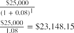where FV is the future value, PV is the present value, r is the interest rate, and n is the number of periods. For example, the first $25,000 is discounted by the equation as follows:

Proof that $23,148.15 will grow to $25,000 in one year at 8% interest:

If we use this same method for each of the five years, increasing the exponent n for each year, we see the result in Table 8.2.

Year	Calculation	Result
1		$23,148.15
2		$21,433.47
3		$19,846.81
4		$18,375.75
5		$17,014.58
TOTAL		$99,818.76

Table 8.2 Present Value of Future Payments

We begin with the amount calculated in our table, $99,818.76. Before any money is withdrawn, a year’s worth of interest at 8% is compounded and added to our balance. Then our first $25,000 is withdrawn, leaving us with $82,804.26. This process continues until the end of five years, when, aside from a minor rounding difference, the fund has “done its job” and is equal to zero. However, we can make this simpler. Because each payment withdrawn (or added, as we will see later) is the same, we can calculate the present value of an annuity in one step using an equation. Rather than the multiple steps above, we will use the following equation:

where PVa is the present value of the annuity and PYMT is the amount of one payment.

In this example, PYMT is $25,000 at the end of each of five years. Note that the greater the number of periods and/or the size of the amount borrowed, the greater the chances of large rounding errors. We have used six decimal places in our calculations, though the actual time value of money factor, combining interest and time, can be much longer. Therefore, our solutions will often use ≅ rather than the equal sign.

By substitution, and then following the proper order of operations:

In both cases, barring a rounding difference caused by decimal expansion, we come to the same result using the equation as when we calculate each of multiple years. It’s important to note that rounding differences can become significant when dealing with larger multipliers, as in the financing of a multimillion-dollar machine or facility. In this text, we will ignore them.

In conclusion, five payments of $25,000, or $125,000 in total, can be funded today with $99,817.81, with the difference being obtained from interest always accumulating on the remaining balance at 8%. The running balance is obtained by calculating the year’s interest on the previous balance, adding it to that balance, and subtracting the $25,000 that is withdrawn on the last day of the year. In the last (fifth) year, just enough interest will accrue to bring the balance to the $25,000 needed to complete the fifth payment.

A common use of the PVa is with large-money lotteries. Let’s assume you win the North Dakota Lottery for

$1.2 million, and they offer you $120,000 per year for 10 years, beginning one year from today. We will ignore taxes and other nonmathematical considerations throughout these discussions and problems. The Lottery Commission will likely contact you with an alternative: would you like to accept that stream of payments … or would you like to accept a lump sum of $787,000 right now instead? Can you complete a money-based analysis of these alternatives? Based purely on the dollars, no, you cannot. The reason is that you can’t compare future amounts to present amounts without considering the effect of time—that is, the time value of money. Therefore, we need an interest rate that we can use as a discounting factor to place these alternatives on the same playing field by expressing them in terms of today’s dollars, the present value. Let’s use 9%. If we discount the future stream of fixed payments (an ordinary annuity, as the payments are identical and they begin one year from now), we can then compare that result to the cash lump sum that the Lottery Commission is offering you instead.

By substitution, and following the proper order of operations:

All things being equal, that expected future stream of ten $120,000 payments is worth approximately $770,119 today. Now you can compare like numbers, and the $787,000 cash lump sum is worth more than the discounted future payments. That is the choice one would accept without considering such aspects as taxation, desire, need, confidence in receiving the future payments, or other variables.

Calculating the Present Value of an Annuity Due

Earlier, we defined an ordinary annuity. A variation is the annuity due. The difference between the two is one period. That’s all—just one additional period of interest. An ordinary annuity assumes that there is a one- period lag between the start of a stream of payments and the actual first payment. In contrast, an annuity due assumes that payments begin immediately, as in the lottery example above. We would assume that you would receive the first annual lottery check of $120,000 immediately, not a year from now. In summary, whether calculating future value (covered in the next section) or present value of an annuity due, the one-year lag is eliminated, and we begin immediately.

Since the difference is simply one additional period of time, we can adjust for this easily by taking the formula for an ordinary annuity and multiplying by one additional period. One more period, of course, is (1 + i). Recall from Time Value of Money I that the formula for compounding is (1 + i)N, where i is the interest rate and N is the number of periods. The superscript N does not apply because it represents 1, for one additional period, and the power of 1 can be ignored. Therefore, faced with an annuity due problem, we solve as if it were an ordinary annuity, but we multiply by (1 + i) one more time.

In our original example from this section, we wished to withdraw $25,000 each year for five years from a fund that we would establish now. We determined how much that fund should be worth today if we intend to receive our first payment one year from now. Throughout this fund’s life, it will earn 8% annually. This time, let’s assume we’ll withdraw our first payment immediately, at point zero, making this an annuity due. Because we’re trying to determine how much our starting balance should be, it makes sense that we must begin with a larger number. Why? Because we’re pulling our first payment out immediately, so less money will remain to start compounding to the amount we need to fund all five of our planned payments! Our rule can be stated as follows:

Whether one is calculating present value or future value, the result of an annuity due must always be larger than that of an ordinary annuity, all other facts remaining constant. Here is the stream of solutions for the example above, but please notice that we will multiply by (1 + i), one additional period, following the same order of operations:

That’s how much we must start our fund with today, before we earn any interest or draw out any money. Note that it’s larger than the $99,817.81 that would be required for an ordinary annuity. It must be, because we’re about to diminish our compounding power with an immediate withdrawal, so we have to begin with a larger amount.

We notice several things:

• The formula must change because the annual payment is subtracted first, prior to the calculation of annual interest.
• We accomplish the same result, aside from an insignificant rounding difference: the fund is depleted once the last payment is withdrawn.
• The last payment is withdrawn on the first day of the final year, not the last. Therefore, no interest is earned during the fifth and final year.

To reinforce this, let’s use the same approach for our lottery example above. Reviewing the facts, you have a choice of receiving 10 annual payments of your $1.2 million winnings, each worth $120,000, and you discount at a rate of 9%. The only difference is that this time, you can receive your first $120,000 right away; you don’t have to wait a year. This is now an annuity due. We solve it just as before, except that we multiply by one additional period of interest, (1 + i):

Again, this result must be larger than the amount we determined when this was calculated as an ordinary annuity.

The calculations above, representing the present values of ordinary annuities and annuities due, have been presented on an annual basis. In Time Value of Money I, we saw that compounding and discounting calculations can be based on non-annual periods as well, such as quarterly or monthly compounding and discounting. This aspect, quite common in periodic payment calculations, will be explored in a later section of this chapter.

Calculating Annuities Used in Structured Settlements

In addition to lottery payouts, annuity calculations are often used in structured settlements by attorneys at law. If you win a $450,000 settlement for an insurance claim, the opposing party may ask you to accept an annuity so that they can pay you in installments rather than a lump sum of cash. What would a fair cash distribution by year mean? If you have a preferred discount rate (the percentage we all must know to calculate the time value of money) of 6% and you expect equal distributions of $45,000 over 10 years, beginning one year from now, you can use the present value of an annuity formula to compare the alternatives:

By substitution:

the lump sum were greater than that, you would likely accept it.

What if you negotiate the first payment to be made to you immediately, turning this ordinary annuity into an annuity due? As noted above, we simply multiply by one additional period of interest, (1 + 0.06). Repeating the last step of the solution above and then multiplying by (1 + 0.06), we determine that

You would insist on that number as an absolute minimum before you would consider accepting the offered stream of payments.

To further verify that ordinary annuity can be converted into an annuity due by multiplying the solution by one additional period’s worth of interest before applying the annuity factor to the payment, we can divide the difference between the two results by the value of the original annuity. When the result is expressed as a percent, it must be the same as the rate of interest used in the annuity calculations. Using our example of an annuity with five payments of $25,000 at 8%, we compare the present values of the ordinary annuity of

$99,817.81 and the annuity due of $107,803.24.

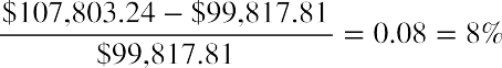
The result shows that the present value of the annuity due is 8% higher than the present value of the ordinary annuity.

Calculating the Future Value of an Annuity

In the previous section, we addressed discounting a periodic stream of payments from the future to the present. We are also interested in how to project the future value of a series of payments. In this case, an investment may be made periodically. Keeping with the definition of an annuity, if the amount of periodic investment is always the same, we may take a one-step shortcut to calculate the future value of that stream by using the formula presented below:

where FVa is the future value of the annuity, PYMT is a one-time payment or receipt in the series, r is the interest rate, and n is the number of periods.

As we did in our section on present values of annuities, we will begin with an ordinary annuity and then proceed to an annuity due.

Let’s assume that you lock in a contract for an investment opportunity at 4% per year, but you cannot make the first investment until one year from now. This is counterintuitive for an investor, perhaps, but because it is the basis of the formula and procedures for ordinary annuities, we will accept this assumption. You plan to invest $3,000 at the end of each year. How much money will you have at the end of five years?

Let’s start by placing this on a timeline like the one appearing earlier in this chapter (see Table 8.3):

Year	0	1	2	3	4	5
Balance Forward ($)	0.00	0.00	3,000.00	6,120.00	9,364.80	12,739.39
Interest Earned ($)		0.00	120.00	244.80	374.59	509.58
Principal Added ($)		3,000.00	3,000.00	3,000.00	3,000.00	3,000.00
New Balance ($)		3,000.00	6,120.00	9,364.80	12,739.39	16,248.97

Table 8.3

As we explained earlier when describing ordinary annuities, the payment for year 1 is not invested until the last day of that year, so year 1 is wasted as a compounding opportunity. Therefore, the amount only compounds for four years rather than five. Also, our fifth payment is not made until the last day of our contract in year 5, so it has no chance to earn a compounded future value. The investor has lost on both ends. In the table above, we have made five calculations, and for a longer-term contract such as 10, 25, or 40 years, this would be tedious. Fortunately, as with present values, this ordinary annuity can be solved in one step because all payments are identical.

Repeating the formula, and then by substitution:

This proof emphasizes that year 1 is wasted, with no compounding because the payment is made on the last day of year 1 rather than immediately. We lose compounding through this ordinary annuity in another way: year 5’s investment is made on the last day of this five-year contract and has no chance to accumulate interest. A more intuitive method would be to enter a contract for an annuity due so that our first payment can be made immediately. In this way, we don’t waste the first year, and all five payments work in year 5 as well. As stated previously, this means that annuities due will yield larger results than ordinary annuities, whether one is discounting (PVa) or compounding (FVa).

Let’s hold all facts constant with the previous example, except that we will invest at the beginning of each year, starting immediately upon locking in this five-year contract. We follow the same technique as in the present value section: we multiply by one additional period to convert this ordinary annuity factor into a factor for an annuity due. Whether one is solving for a future value or a present value, the result of an annuity due must always be larger than an ordinary annuity. With future value, we begin investing immediately, so the result will be larger than if we waited for a period to elapse. With present value, we begin extracting funds immediately rather than letting them work for us during the first year, so logically we would have to start with more.

Continuing our example but converting it to an annuity due, we will multiply by one additional period, (1 + i). All else remains the same:

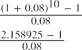
Let’s provide one additional example of each. Assume that you have a chance to invest $15,000 per year for 10 years, earning 8% compounded annually. What amount would you have after the 10 years? If we can only make our first payment at the end of each year, our ending value will be

each following year, we modify the formula above by multiplying the annual payment by one additional period:

THINK IT THROUGHBegin an Investing Program at Age 20 or 30?In this chapter’s introductory section, Why It Matters, we posed a question about pledging to invest $1,000 each year until you reach age 60. If you can earn a 5% annual rate of interest, how much will you have if you begin at age 20? What if you delay this program until age 30? The additional 10 years can make a surprisingly large difference. How can you calculate that difference?Solution:Perform two separate calculations comparable to the chapter examples above, using the formula for the future value of an ordinary annuity. You plan to make the first investment immediately, making this an annuity due, so you will multiply by one additional period, (1 + 0.05). Notice that the only difference between the two calculations is the exponent N, representing the number of periods.Thirty years (starting at age 30):Forty years (starting at age 20):Waiting 10 years before committing to this program comes with a surprisingly high cost—a loss of almost 82% of the potential value.

How Annuities Are Used for Retirement Planning

On a final note, how might annuities be used for retirement planning? A person might receive a lump-sum windfall from an investment, and rather than choosing to accept the proceeds, they might decide to invest the sum (ignoring taxes) in an annuity. Their intention is to let this invested sum produce annual distributions to supplement Social Security payments. Assume the recipient just received $75,000, again ignoring tax effects. They have the chance to invest in an annuity that will provide a distribution at the end of each of the next five years, and that annuity contract provides interest at 3% annually. Their first receipt will be one year from now. This is an ordinary annuity.

We can also solve for the payment given the other variables, an important aspect of financial analysis. If the person with the $75,000 windfall wants this fund to last five years and they can earn 3%, then how much can they withdraw from this fund each year? To solve this question, we can apply the present value of an annuity formula. This time, the payment (PYMT) is the unknown, and we know that the PVa, or the present value that they have at this moment, is $75,000:

The person can withdraw this amount every year beginning one year from now, and when the final payment is withdrawn, the fund will be depleted. Interest accrues each year on the beginning balance, and then

$16,376.60 is withdrawn at the end of each year.

LINK TO LEARNINGAnother View of AnnuitiesMany examples of annuities are available, with presentations as varied as the opinions as to how appropriate they are for investors, especially retirees. Math Is Fun (https://openstax.org/r/Math_Is_Fun) is particularly interesting and potentially helpful for understanding how to apply this knowledge.

8.3
Loan Amortization

Learning Outcomes

By the end of this section, you will be able to:

• Distinguish between different types of loans.
• Explain how amortization works.
• Create an amortization schedule.
• Calculate the cost of borrowing.

Types of Loans

Funds can be loaned to businesses of any type, including corporations, partnerships, limited liability companies, and proprietorships. Bankers often refer to these lending structures as facilities, and they can be tailored to the specific needs of the borrower in a number of ways. Similarly, lenders develop loans and lines of credit for individuals. Whether for a business or an individual, the purpose of the loan, method of repayment, interest rate, specific terms, and time involved must all be tailored to the goals of the borrower and the lender. In this chapter, we will focus on fixed-rate loans, although other alternatives exist.

Typical business loans include the following:

• Term loans generally bear a maturity date and a set rate of interest and are typically used to finance investments in assets such as equipment, buildings, and possibly other acquired firms. The length of the term loan is generally designed to match the useful life of the asset being financed, and it will usually be repaid on a monthly schedule. It’s common for a term loan to be backed by collateral, such as the asset itself or other assets of the business.
• Revolving lines of credit (revolvers), are used to finance the short-term working capital needs of a business. Revolvers will have a specific maximum but no set schedule of monthly payments. Interest accrues on the amount of cash that a company has drawn down from the facility. These credit lines may be secured by accounts receivable, inventory, other assets of the business, or sometimes simply the good

faith and credit of the company if the firm is strong, creditworthy, and established with the lender. Revolvers must often be fully repaid and unused for a short period of time to assure the lender that the borrower is not using this facility for longer-term needs.

Personal loans also come in several types, designed for the purpose the borrower (consumer) has in mind, with assistance from the lender in determining the appropriate structure:

• Personal lines of credit are similar to lines of credit on bank cards, with interest being charged on the outstanding balance of the credit line. These are available on the basis of personal credit scores, with data being supplied by the three best-known credit reporting firms: Experian, Equifax, and TransUnion. Individuals should check their scores with each of these companies at least once per year, which they can do for no charge. Additional requests from the same company require a small fee.
• An unsecured personal loan is an installment loan, initially drawn for a fixed amount and repaid on a periodic schedule with interest, as we have seen in our annuity examples. Unsecured means that the loan is not secured by collateral but is instead based on the strong credit history of the borrower.
• In contrast, a secured personal loan has an asset backing up the unpaid amount, and if the consumer defaults on the debt, the asset can be seized by the lender to satisfy their claim. A common example is an auto loan, which is secured by the car being purchased; nonpayment or default on the loan can lead to the borrower’s car being repossessed.
• A mortgage loan is another type of secured personal loan, but for a longer period, such as 20, 25, or even 30 years. The home being purchased or built is the collateral, and the home may be foreclosed upon if the borrower defaults. Full title to the home typically remains with the lender as long as an unpaid balance remains on the debt.
• Student loans are borrowings intended to fund college or career education, and they can come from a financial institution or the federal government. Interest rates on these loans are generally low and advantageous, and repayment does not begin until after the borrower’s education is complete (or if they drop below a certain level of time status, such as becoming a half-time student).

Calculating Loan Payments Using Simple Amortization

Loan amortization refers to a schedule of how and when a debt will be repaid with interest. As noted, we will focus on fixed-rate debts, such as auto loans, personal loans with installment payments, or mortgages. Before entering into a borrowing agreement, the borrower can use any of a number of tools to verify the terms being offered, such as the monthly payment on a car loan financed by the dealer. In many cases, this is accomplished by using the present value of an annuity formula:

We’ve already reviewed the present value of ordinary annuities in several examples. Before we look into business or consumer loans and their repayment, we must review an area of Time Value of Money I.

We’re not likely to make annual payments on a home mortgage or auto loan, as these are commonly paid on a monthly basis. Fortunately, our formulas are easily adjusted from annual to non-annual periods. You will recall that we solve for non-annual periods in the same way, with two adjustments: (1) we divide the annual interest rate by the number of periods in the year, and (2) we multiply the time periods by the number of those periods within a year. Therefore, in the case of monthly debt service, including interest and principal, we use 12 periods.

Given a three-year car loan at 6%, rather than using 6% and 3 periods in our formula, we would instead use 0.5% (6% ÷ 12) and 36 periods (3 years × 12), and then apply the present value of an annuity formula in the same way. Let’s say the three-year, 6% auto loan is for $32,000. You need to know if you can squeeze the monthly payment into your budget. For our examples, we will ignore any other charges, fees, taxes, or extras that your lender might include in these payments, and we will focus only on interest and principal repayment.

You will make the first payment one month from now, making this an ordinary annuity. What is the amount of your monthly debt service? In this case, you would be solving for a different unknown: the payment amount.

By substitution into the present value of an annuity formula, adjusting for monthly payments as noted:

Dividing both sides by 32.781 to isolate the payment amount (PYMT) gives us

Solving for the payment, we find that it’s approximately $973.50 per month. You consult your monthly budget and find that you can cover this monthly payment, so you conclude the deal. Ask the salesperson for the amortization table on this debt to show how your 36 payments of $973.50 will cover your interest plus repayment of the principal amount of the debt. At this point, you know how to complete your own table. Using a financial calculator or Microsoft Excel simplifies the operation above to a few keystrokes, as presented later in this chapter.

…continued…
Two extracts from an amortization table are shown in Table 8.4.

Month	Payment	Interest	Principal	Remaining Balance
1	973.50	160.00	813.50	31,186.50
2	973.50	155.93	817.57	30,368.93
3	973.50	151.84	821.66	29,547.27
4	973.50	147.74	825.77	28,721.51
5	973.50	143.61	829.89	27,891.61

33	973.50	19.23	954.27	2,891.54
34	973.50	14.46	959.04	1,932.50
35	973.50	9.66	963.84	968.66
36	973.50	4.84	968.66	0.00
Total	35,046.00	3,046.08	32,000.00

Table 8.4 Extracts from an Amortization Table ($)

This table resembles proofs we have seen of annuities, but let’s focus on some details:

• Each fixed payment contains both interest and principal repayment.
• Because the payments are fixed and the amount of remaining debt is decreasing, the monthly interest portion is always decreasing, and the amount of principal payment therefore must be increasing.

We can conclude that the lender is making more of their revenue (interest) in the early months than in the later months. In addition, the debt is decreasing slowly in the early months and more rapidly in the later

months. We can all agree that lenders are compensated for the risks they take earlier rather than later. Of the 36 payments of $973.50, $32,000 has been repaid as the principal borrowed. The remaining $3,046.08 is the lender’s revenue, the cost of credit.

For an additional example, one that drives home the point that more interest is paid in the early months of a long-term loan, we will consider a 20-year home mortgage. Home mortgage payments are typically made monthly, and again, we will ignore additional charges by the lender, such as real estate tax and homeowner’s insurance. Let’s assume you buy a $200,000 home, pay $60,000 as a cash deposit, and will finance the remaining $140,000 over 20 years. The bank offers you a 3.6% annual interest rate. What will the amount of your monthly payment be for the interest and principal repayment? The bank will tell you, of course, but let’s prove it for ourselves. We’ll do it in exactly the same fashion as the car loan above, using the present value of an annuity formula. Remember that you are not financing the entire $200,000 purchase; you pay $60,000 in cash, so you are only financing the remaining $140,000.

We modify the periods from years to months by multiplying by 12, and we modify the annual rate to a monthly rate by dividing by 12, resulting in

By substitution into the present value of an annuity formula:

We divide both sides by 170.907667 to isolate the payment amount (PYMT):

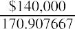
Your monthly mortgage payment is $819.16. As in our auto loan example, we’ll complete an amortization table of our own—though, of course, you’ll remember to ask your lender for their version. Extracts from a full

240-month table are shown in Table 8.5 below. The front-end packing of interest revenue is more obvious here because of the longer time period.

Month	Payment	Interest	Principal	Remaining Balance
				140,000.00
1	819.16	420.00	399.16	139,600.84
2	819.16	418.80	400.36	139,200.48
3	819.16	417.60	401.56	138,798.92
4	819.16	416.40	402.76	138,396.16
5	819.16	415.19	403.97	137,992.19
6	819.16	413.98	405.18	137,587.01
7	819.16	412.76	406.40	137,180.61

Table 8.5 Amortization Table for a Mortgage ($)

Month	Payment	Interest	Principal	Remaining Balance
8 9	819.16 819.16	411.54 410.32	407.62 408.84	136,772.99 136,364.15

236	819.16	12.17	806.99	3,250.84
237	819.16	9.75	809.41	2,441.44
238	819.16	7.32	811.84	1,629.60
239	819.16	4.89	814.27	815.33
240	819.16	2.45	816.71	(1.38)

…continued….Total 196,598.40 56,597.02 140,001.38(Rounding)




Table 8.5 Amortization Table for a Mortgage ($)

As with your car loan, earlier payments contain more interest than loan repayment, so the lender’s revenue is at a significant peak in the early years. The length of the loan, coupled with the frequent compounding, emphasizes this. In month 10, the interest and principal amounts “pass” each other, and now the loan balance is dropping at a quicker rate. Finally, note that you will pay more than $56,000 to finance this $140,000 borrowing. If you pay off this mortgage over 240 months as planned, the interest cost represents an additional 28% of the full cost of the home!

If the borrower has the means to make an accelerated payment against this debt—for example, due to a bonus or other windfall—doing so can make a significant difference in the total cost of financing over the life of the loan. Assume that after three years (month 36), you receive a bonus of $2,000 and decide to apply the entire amount to prepay the remaining balance. Your loan agreement allows you to apply the entire amount to the remaining unpaid balance of the mortgage. While this might seem equal to just 2.5 months’ worth of payment, the debt is fully paid off almost 6 months ahead of schedule, and total interest is reduced from over

$56,000 to $55,000. The ability to prepay long-term debts such as this is clearly worth negotiating initially.

8.4
Stated versus Effective Rates

Learning Outcomes

By the end of this section, you will be able to:

• Explain the difference between stated and effective rates.
• Calculate the true cost of borrowing.

The Difference between Stated and Effective Rates

If you look at the bottom of your monthly credit card statement, you could see language such as “The interest rate on unpaid balances is 1.5% per month.” You might think to yourself, “So, that’s 12 months times 1.5%, or 18% per year.” This is a fine example of the difference between stated and effective annual interest rates. The effective interest rate reflects compounding within a one-year period, an important distinction because we tend to focus on annual interest rates. Because compounding occurs more than once per year, the true annual rate is higher than appears. Please remember that if interest is calculated and compounded annually, the stated and effective interest rates will be the same. Keep in mind that the following principles work whether you are the debtor paying off an obligation or an investor hoping for more frequent compounding. The dynamics of the time value of money apply in either direction.

Effective Rates and Period of Compounding

Let’s remain with our example of a credit card statement that indicates an interest rate of 1.5% per month on

unpaid balances. If you use this card only once, to make a $1,000 purchase in January, and then fail to pay the bill when it comes due, the issuer will bill you $15. Now you owe them $1,015. Assume you completely ignore this bill and never pay it throughout the rest of the year. The monthly calculation of interest starts to compound on past interest assessments in addition to the $1,000 initial purchase (see Table 8.6).

Month Interest Balance
		1,000.00
1	15.00	1,015.00
2	15.23	1,030.23
3	15.45	1,045.69
4	15.69	1,061.36
5	15.92	1.077.28
6	16.16	1,093.44
7	16.40	1,109.84
8	16.65	1,126.49
9	16.90	1,143.39
10	17.15	1,160.54
11	17.41	1,177.95
12	17.67	1,195.62

Table 8.6 Compounded Interest on a Credit Card Statement ($)

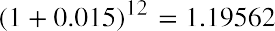
Because interest compounds monthly rather than annually, the effective annual rate is 19.56%, not the intuitive rate of the stated 1.5% times 12 months, or 18%. Our basic compounding formula of (1+i)^n by substitution shows:

To isolate the effective annual rate, we then deduct 1 because our interest calculations are based on the value of $1:

Therefore, it falls to the consumer/borrower to understand the true cost of borrowing, especially when larger dollar amounts are involved. If we had been dealing with $10,000 rather than $1,000, the annual difference would be more than $156.

LINK TO LEARNINGA Helpful Demonstration . . .From the Corporate Finance Institute (https://openstax.org/r/Corporate_Finance_Institute) comes a fine visual of a similar example. Here, we see the effective annual rate that results from taking a nominal annual rate of 12%, with a benefit to an investor if they have the benefit of monthly compounding.

One example of the importance of understanding effective interest rates is an invention from the early 1990s:

the payday advance loan (PAL). The practice of offering such loans can be controversial because it can lead to very high rates of interest, perhaps even illegally high, in an act known as usury. Although some states have outlawed PALs and others place limits on them, some do not. A PAL is a short-term loan in anticipation of a person’s next paycheck. A person in need of money for short-term needs will write a check on Thursday but date the check next Thursday, which is their normal payday; assume this transaction is for $200. The lender, typically operating from a storefront, will advance the $200 cash and hold the postdated check. The lender charges a fee—let’s say $14—as their compensation. The following Thursday, the borrower is expected to pay off the advance, and if they do not, the lender can deposit the postdated check. If that check has insufficient funds, more fees and penalties will likely be assessed.

One primary reason that arrangements such as these are controversial is the excessively high nominal (stated) interest rate that they can represent. For a one-week loan of $200, the borrower is paying $14, or 7% of the borrowed amount. If this is annualized, with 52 seven-day periods in a year, the stated rate is 364%! While a PAL might seem to be an effective immediate solution to a cash shortfall, the mathematics behind the true cost of borrowing simply do not make sense, and a person who uses such arrangements regularly is placing themselves at a dreadful financial disadvantage.

THINK IT THROUGHHow Tempting Is That Refund Anticipation?Refund anticipation loans (RALs) began in 1987, and they are still available (though not from banks) and used by millions of people.1 Now, RALs come from private lending chains. These loans allow you to determine your April 15 personal income tax liability through a preparer and receive an advance against your expected refund.2 But beware: your ability to analyze the true cost of money is always critical. Like all loans, RALs bear a rate of interest. Let’s assume that the firm that prepared your tax return determines that you’re entitled to an $800 refund. Once they advance that amount to you, it will bear interest at a certain rate; we’ll assume 0.5% per week. You might expect a tax refund in four weeks. Half a percent of $800 doesn’t sound like much, but what happens when you annualize it into an effective rate, assuming your tax refund arrives exactly four weeks from when you accept the loan? Assume no compounding during those four weeks.Solution:A weekly rate of 0.5% on the $800 advance is $4 per week, so for four full weeks, you’ve paid $16 for the use of $800. Of course, that totals 2% of the amount advanced. There are 13 four-week periods in a year, so even though the interest rate appears to be small, it amounts to 26% when annualized! We assumed no compounding to keep the illustration simple, but we further assume that you are not using this advance throughout the year. If you were, then periodic compounding would drive the effective rate even higher, to just over 29.3%.

• Michelle Singletary. “Another Reason Not to Opt for a Tax Refund Loan: It May Delay Your Next Stimulus Payment.” Washington Post, February 16, 2021. https://www.washingtonpost.com/business/2021/02/16/tax-refund-loan-problems/
• Amelia Josephson. “What Is a Refund Anticipation Loan?” SmartAsset. March 18, 2021. https://smartasset.com/taxes/what-is-a- refund-anticipation-loan

8.5
Equal Payments with a Financial Calculator and Excel

Learning Outcomes

By the end of this section, you will be able to:

• Use a financial calculator and Excel to solve perpetuity problems.
• Use a financial calculator and Excel to solve annuity problems.
• Calculate an effective rate of interest.
• Schedule the amortization of a loan repayment.

Solving Time Value of Money Problems Using a Financial Calculator

Since the 1980s, many convenient and inexpensive tools have become available to simplify business and personal calculations, including personal computers with financial applications and handheld/desktop or online calculators with many of the functions we’ve studied already. This section will explore examples of both, beginning with financial calculators. While understanding and mastery of the use of time value of money equations are part of a solid foundation in the study of business and personal finance, calculators are rapid and efficient.

We’ll begin with the constant perpetuity that we used to illustrate the constant perpetuity formula. A share of preferred stock of Shaw Inc., pays an annual $2.00 dividend, and the required rate of return that investors in this stock expect is 7%. The simple technique to solve this problem using the calculator is shown in Table 8.7.

StepDescriptionEnterDisplaySet all variables to defaults 2ND [RESET] ENTER RST 0.00Enter formula2 ÷ 7 % =28.57

Table 8.7 Calculator Steps to Find the Required Rate of Return³

Earlier we solved for the present value of a 5-year ordinary annuity of $25,000 earning 8% annually. We then solved for an annuity due, all other facts remaining the same. The two solutions were $99,817.50 and

$107,802.50, respectively. We enter our variables as shown in Table 8.8 to solve for an ordinary annuity:

Step12345DescriptionSet all variables to defaults Enter number of paymentsEnterDisplay2ND [RESET] ENTER RST5 NEnter interest rate per payment period 8 I/YN =I/Y =0.005.008.00Enter payment amountCompute present value25000 +/- PMTCPT PVPMT = -25,000.00PV =99,817.75

Table 8.8 Calculator Steps to Solve for an Ordinary Annuity

Note that the default setting on the financial calculator is END to indicate that payment is made at the end of a period, as in our ordinary annuity. In addition, we follow the payment amount of $25,000 with the +/- keystroke—an optional step to see the final present value result as a positive value.

To perform the same calculation as an annuity due, we can perform the same procedures as above, but with two additional steps after Step 1 to change the default from payments at the end of each period to payments at the beginning of each period (see Table 8.9).

• The specific financial calculator in these examples is the Texas Instruments BA II PlusTM Professional model, but you can use other financial calculators for these types of calculations.

StepDescriptionEnterDisplay
1Set all variables to defaults	2ND [RESET] ENTER	RST	0.00
2Change default to payment at end of period 2ND [BGN] 2ND [SET] BGN0.00
3Return to calculator mode	2ND [QUIT]		0.00
4Enter number of payments	5 N	N =	5.00
5Enter interest rate per payment period	8 I/Y	I/Y =	8.00
6Enter payment amount	25000 +/- PMT	PMT =	-25,000.00
7Compute present value	CPT PV	PV =	107,803.17

Table 8.9 Calculator Steps to Solve for an Annuity Due

The procedures to find future values of both ordinary annuities and annuities due are comparable to the two procedures above. We begin with the ordinary annuity, with reminders that this is the default for the financial calculator and that entering the payment as a negative number produces a positive result (see Table 8.10).

Step12345DescriptionSet all variables to defaults Enter number of paymentsEnterDisplay2ND [RESET] ENTER RST5 NEnter interest rate per payment period 4 I/YN =I/Y =0.005.004.00Enter payment amountCompute future value3000 +/- PMTCPT FVPMT = -3,000.00FV =16,248.97

Table 8.10 Calculator Steps to Find the Future Value of an Ordinary Annuity

Solving for an annuity due with the same details requires the keystrokes listed in Table 8.11.

Step1234567DescriptionSet all variables to defaultsEnter2ND [RESET] ENTERDisplayRSTChange default to payment at end of period 2ND [BGN] 2ND [SET] BGNReturn to calculator mode Enter number of paymentsEnter interest rate per payment period Enter payment amountCompute future value2ND [QUIT]5 N4 I/Y3000 +/- PMT CPT FVN =I/Y =0.000.000.005.004.00PMT = -3,000.00FV =16,898.93

Table 8.11 Calculator Steps to Find the Future Value of an Annuity Due

Earlier in the chapter, we explored the effect of interannual compounding on the true cost of money, recalling the basic compounding formula:

We saw that when modified for monthly compounding at a stated rate of 1.5%, the actual (effective) rate of interest per year was 19.56%. One simple way to prove this is by using the calculator keystrokes listed in Table

8.12.

Step12345DescriptionSet all variables to defaultsEnter2ND [RESET] ENTERDisplayRST0.00Set the display to four decimal places 2ND [FORMAT] 4 ENTER DEC = 4.0000Return to calculator modeEnter (1 + the monthly interest rate) Enter the number of months2ND [QUIT]1.015 YX12 YX0.00001.01501.1956

Table 8.12 Calculator Steps to Prove the Actual Rate of Interest per Year

Had we assumed that the stated monthly interest rate of 1.5% could be simply multiplied by 12 months for an annual rate of 18%, we would be ignoring the effect of more frequent compounding. As indicated above, the annual interest on the money that we spent initially, accumulating at a rate of 1.5% per month, is 19.56%, not 18%:

The final example in this chapter will represent the amortization of a loan. Using a 36-month auto loan for

$32,000 at 6% per year compounded monthly, we can easily find the monthly payment and the amortization of this loan on our calculator using the following procedures and keystrokes.

First, we find the monthly payment (see Table 8.13).

Step	Description	Enter	Display
1	Set all variables to defaults	2ND [RESET] ENTER	RST0.00
2	Set payments per year to 12	2ND [P/Y] 12 ENTER	P/Y =12.00
3	Return to calculator mode	2ND [QUIT]	0.00
4	Enter number of payments with the payment multiplier	3 2ND [xP/Y] N	N =36.00
5	Enter annual interest rate	6 I/Y	I/Y =6.00
6	Enter loan amount	32000 PV	PV =32,000.00
7	Compute the monthly payment	CPT PMT	PMT =-973.50

Table 8.13 Calculator Steps to Find the Monthly Payment of a Loan

We’ve verified the amount of our monthly debt service, including both the interest and repayment of the principal, as $973.50. The next step with our calculator is to verify our amortization at any point (see Table 8.14).

Step	Description	Enter	Display
1	Set previous work as an amortization worksheet	2ND [AMORT]	P1 =1.00
2	Set beginning period to 1	1 ENTER	P1 =1.00
3	Set ending period to 12	↓ 12 ENTER	P2 =12.00
4	Display amortization data at the end of month 12	↓	BAL = 21,965.02
5		↓	PRN = -10,034.98

Table 8.14 Calculator Steps to Verify Amortization at the End of One Year

Step	Description	Enter	Display
6		↓	INT =	-1,647.02

Table 8.14 Calculator Steps to Verify Amortization at the End of One Year

Without resetting the calculator, we will try a second example, this time reviewing the second full year of amortization at the end of 24 months (see Table 8.15).

Step123456DescriptionEnterDisplaySet previous work as an amortization worksheet 2ND [AMORT] P1 =Change beginning period to month 13Change ending period to month 2413 ENTER↓ 24 ENTERDisplay amortization data at the end of month 24 ↓↓↓P1 =P2 = BAL =1.0013.0024.0011,311.13PRN = -10,653.89INT =-1,028.11

Table 8.15 Calculator Steps to Verify Amortization at the End of Two Years

Solving Time Value of Money Problems Using Excel

Microsoft’s popular spreadsheet program Excel is arguably one of the most common and powerful numeric and data analysis products available. Yet while mastery of Excel requires extensive study and practice, enough basics can be learned in two or three hours to provide the user with the ability to solve problems quickly and conveniently, including extensive financial capability. Most of the calculations in this chapter were prepared with Excel.

The boxes in the Excel gridwork, known individually as cells (located at the intersection of a column and a row), can contain numbers, text, and very powerful formulas (or functions) for calculations and data analytics. Cells, rows, columns, and groups of cells (ranges) are easily moved, formatted, and replicated. In the mortgage amortization table for 240 months seen in Section 8.3.2, only the formulas for month 1 were typed in. With one simple command, that row of formulas was replicated 239 more times, with each line updating itself with relevant number adjustments automatically. With some practice, a long table such as that can be constructed by even a relatively new user in less than 10 minutes.

In this section, we will illustrate how to use Excel to solve problems from earlier in the chapter, including perpetuities, ordinary annuities, effective interest rates, and loan amortization. We will omit the basic dynamics of an Excel spreadsheet because they were presented sufficiently in preceding chapters.

Revisiting the constant perpetuity from Section 8.1, in which our shares of Shaw Inc., preferred stock pay an annual fixed dividend of $2.00 and the required rate of return is 7%, we do not use an Excel function for this simple operation. The two values are entered in cells B3 and B4, respectively.

We enter a formula in cell B6 to perform the division and display the result in that cell. The actual contents of cell B6 are typed below it for your reference, in cell B8 (see Figure 8.2).

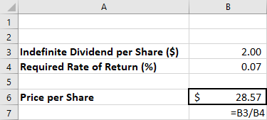
Figure 8.2 Excel Spreadsheet for Valuing a Perpetuity

Download the spreadsheet file (https://openstax.org/r/spreadsheet_file_Chapter08_finance) containing key Chapter 8 Excel exhibits.

To find the present value of an ordinary annuity, we revisit Section 8.2.1. You will draw $25,000 at the end of each year for five years from a fund earning 8% annually, and you want to know how much you need in that fund today to accomplish this. We accomplish this in Excel easily with the PV function. The format of the PV command is

=PV(rate,periods,payment,0,0)

Only the first three arguments inside the parentheses are used. We’ll place them in cells and refer to those cells in our PV function. As an option, you could also type the numbers into the parentheses directly. Notice the slight rounding error because of decimal expansion. Also, the payment must be entered as a negative number for your result to be positive; this can be accomplished either by making the $25,000 in cell B5 a negative amount or by placing a minus sign in front of the B5 in the formula’s arguments. In cell B3, you must enter the percent either as 0.08 or as 8% (with the percent sign). We repeated the formula syntax and the actual formula inputs in column A near the result, for your reference (see Figure 8.3).

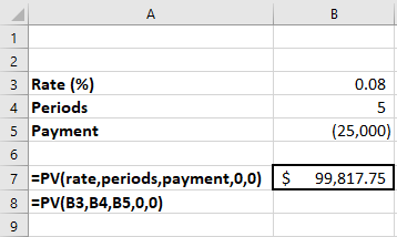
Figure 8.3 Excel Spreadsheet Showing the Present Value of an Ordinary Annuity

We also found the present value of an annuity due. We use the same information from the ordinary annuity problem above, but you will recall that the first of five payments happens immediately at the start of year 1, not at the end. We follow the same procedures and inputs as in the previous example, but with one change to the PV function: the last argument in the parentheses will change from 0 to 1. This is a toggle switch that commands the PV function to treat this as an annuity due instead of an ordinary annuity (see Figure 8.4).

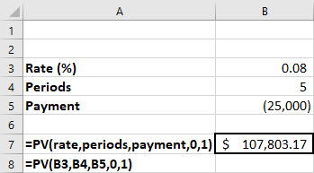
Figure 8.4 Excel Spreadsheet Showing the Present Value of an Annuity Due

Section 8.2 introduced us to future values. Comparable to the PV function above, Excel provides the FV function. Using the same information—$3,000 invested annually for five years, starting one year from now, at 4%—we’ll solve using Excel (see Figure 8.5). The format of the command is

=FV(rate,periods,payment,0,0)

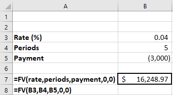
Figure 8.5 Excel Spreadsheet Showing the Future Value of an Ordinary Annuity

As with present values, using the same data but solving for an annuity due requires the fifth argument inside the parentheses to be changed from 0 to 1; all other values remain the same (see Figure 8.6).

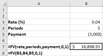
Figure 8.6 Excel Spreadsheet Showing the Future Value of an Annuity Due

In Section 8.4, we explained the difference between stated and effective rates of interest to show the true cost of borrowing, in this case for a one-year period, if interest is compounded for periods within a year. The syntax for the Excel effect function to calculate this rate is

=EFFECT(rate,periods)

where rate is the nominal rate and periods represents the number of periods within a year.

Earlier, our example showed that 1.5% compounded monthly results in not 18% per year but actually over 19.56% (see Figure 8.7).

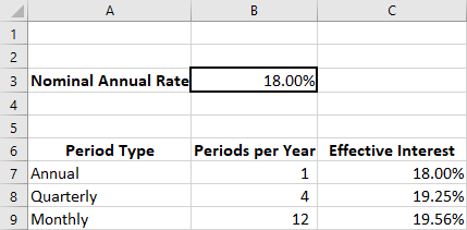
Figure 8.7 Excel Spreadsheet Showing Effective Interest Rate

Note several things: First, the nominal interest rate is entered as a percent. Second, the actual effect function in C7 is typed as =EFFECT(rate,B7); we use the word rate because we actually assigned a name to cell B3, so Excel can use it in a function and replicate it without it changing. When cell C7 is replicated to C8 and C9, rate remains the same, but the formulas automatically adjust to use B8 and B9 for the periods.

To assign a name to a cell, keep in mind that every cell has column-row coordinates. We want cell B3 to be the anchor of our effective rate calculations. Rather than referring to cell B3, we can name it, and in this case, we use the name rate, which we can then use in formulas like any other Excel cell letter-number reference. Place the cursor in cell B3. Now, look at cell A1 on the grid: right above that cell, you see a box displaying B3, the current cursor location. If you click in that box and type “rate” (without the quotation marks), as we did, then hit the enter key, the value in that box will change to rate. Now, if you type “rate” (again, without quotation marks) into a formula, Excel knows to use the contents of cell B3.

Excel provides convenient tools for figuring out amortization. We’ll revisit our 36-month auto loan for $32,000 at 6% per year, compounded monthly. A loan amortization table for a fixed interest rate debt is usually formatted as follows, with the Interest and Principal columns interchangeable:

PeriodPaymentInterestPrincipalBalance

In Excel, a table is completed by using the function PMT. The individual steps follow.

• List the information about the loan in the upper left of the worksheet, and create the column headings for the schedule of amortization. Type “B5” (without the quotation marks) in cell E9 to begin the schedule. Then enter 1 for the first month under the Payment # (or Month) column, in cell A10 (see Figure 8.8).

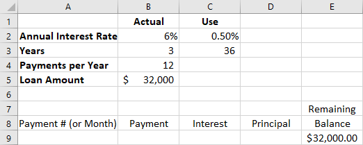
Figure 8.8 Step 1 of Creating an Amortization Table

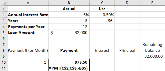• Next, in cell B10, the payment is derived from the formula =PMT(rate,periods,pv), with PV representing the present value, or the loan amount. Because we are compounding monthly, enter C$2 and C$3 for the rate and periods, respectively. Cell B5 is used for the loan amount, but notice the optional minus sign placed in front of the entry B$5; this causes the results in the schedule to be displayed as positive numbers. The dollar sign ($) inserted in the cell references forces Excel to “freeze” those locations so that they don’t attempt to update when we replicate them later; this is known in spreadsheet programs as an absolute reference (see Figure 8.9).

Figure 8.9 Step 2 of Creating an Amortization Table

• The next step is to calculate the interest. We take the remaining balance from the previous line, in this case cell E9, and multiply it by the monthly interest rate in cell C2, typing C$2 to lock in the reference. The remaining balance of the loan should always be multiplied by this monthly percentage (see Figure 8.10).

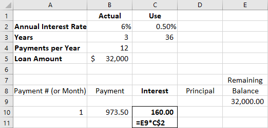
Figure 8.10 Step 3 of Creating an Amortization Table

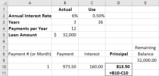• Because this is a fixed-rate loan, whatever is left from each payment after first deducting the interest represents principal, the amount by which the balance of the outstanding loan balance is reduced. Therefore, the contents of cell D10 represent B10, the total payment, minus C10, the interest portion (see Figure 8.11). No dollar signs are included because this cell reference can adjust to each row into which this formula is replicated, as will be seen in the following examples.

Figure 8.11 Step 4 of Creating an Amortization Table

• Because our principal portion of the last payment has reduced our outstanding balance, it is subtracted from the preceding balance in cell E9 (see Figure 8.12). The command therefore is =E9-D10.

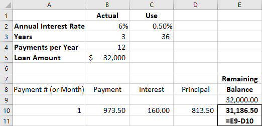
Figure 8.12 Step 5 of Creating an Amortization Table

Now that the first full row is defined, an amortization schedule is easily developed by Excel’s replication abilities. Place the cursor on cell A10, hold down the left mouse button, and drag the cursor to cell E10. Cells A10 through E10 in row 10 should now be highlighted. Release the mouse button. Then “grab” the tiny square symbol at the bottom right of cell E10 and drag it downward as far as you need; in this case, you’ll need 35 more rows because this is a 36-month loan, so it will end at row 45. We added a line for totals.

This is now a complete loan amortization schedule (see Figure 8.13). The first several periods display, followed by the last few periods, to prove that the schedule is complete (data rows for month 4 to month 22 are hidden).

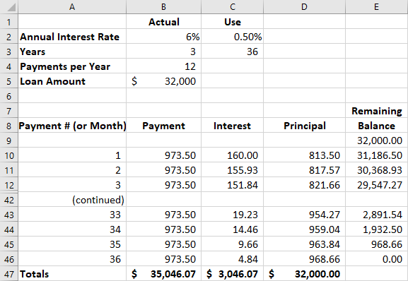
Figure 8.13 Completed Amortization Schedule

This will look familiar; it’s the same amortization table used as a proof in Section 8.3 (see Table 8.4). There is no rounding error because Excel uses the full decimal expansion in its calculations.

This chapter has explored the time value of money by expanding on the concepts discussed in Time Value of Money I with additional funds being periodically added to or subtracted from our investment, either compounding or discounting them according to the situation. In all cases, the payments in the stream were identical. If they had not been identical, a separate set of operators would be required, and these will be addressed in the next chapter.

Summary

Perpetuities

A perpetuity is an investment that is intended to provide an expected return indefinitely, either remaining constant or growing by an incremental amount. Preferred stock is a common example with a preestablished dividend formula. An indefinite stream of payments cannot be compounded into a future value, but it can be discounted to a present value, providing an opportunity to determine the amount an investor should be willing to pay for a share of that stock.

Annuities

An annuity is a stream of fixed periodic payments that is expected to be paid or received. Calculations of future value or present value are commonly performed on these payment streams for a wide number of reasons in business and personal financial analysis, as seen in the chapter focusing on single amounts, particularly in loan repayment. Annuities may be ordinary annuities, in which the first cash flow of a series occurs at the end of the first period, or annuities due, if the first cash flow occurs at the beginning point of the first period.

Loan Amortization

Loans are contracts between a lender and a borrower. Failure to observe the rules of that contract, such as payment of interest or repayment of the amount owed, can subject the borrower to substantial penalties as well as damage to their credit. Loan agreements bearing a fixed rate of interest have a scheduled amortization, or rate and time of repayments with interest. Several types of business and personal loans were described.

Stated versus Effective Rates

For a borrower to understand the true cost of financing, they must be familiar with interannual compounding, which can cause a stated interest rate that appears to be annual to actually be higher. The effective rate of interest was demonstrated to understand that true cost.

Equal Payments with a Financial Calculator and Excel

The use of two tools for managing and understanding the time value of money and its many applications was discussed: a professional financial calculator and the popular Microsoft Office Suite spreadsheet application Excel.

Key Terms

annuity a stream of regular, periodic payments to be received or paid

annuity due a stream of periodic payments in which the payment or receipt occurs at the beginning of each period

constant perpetuity a stream of periodic payments that is expected to continue indefinitely with no change in the amount paid or received

discount rate an interest rate used in time value of money calculations to determine present value; may derive from several sources, such as stated contract rates, costs to borrow, or expected rates of return on investments

effective interest rate the interest rate that results when compounding occurs multiple times within a year; the true cost of borrowing

growing perpetuity a stream of periodic payments that is expected to continue indefinitely with growth of the amount paid or received in the future, usually by a fixed percentage

loan amortization the scheduling of periodic repayment of a debt, typically involving regular payments or receipts of amounts that include both interest payment and repayment of the principal of the amount owed

lump sum a single cash payment made in lieu of a series of future payments, such as a lottery payout or a

legal settlement

ordinary annuity a stream of periodic payments in which the payment or receipt occurs at the end of each period

perpetuity a stream of periodic payments that is expected to continue indefinitely

preferred stock shares of ownership in a corporation that typically entitle the holder to a fixed dividend per share, if declared by the corporation, with priority over holders of that corporation’s common stock

required rate of return the minimum amount of return that an investor will accept on an investment given the level of risk involved

retirement planning the process of determining one’s objectives for retirement, including one’s finances, and developing strategies and tactics to achieve them

structured settlements monetary legal settlements that are paid out in installments, such as an annuity, rather than a lump sum cash amount