6 Lesson 4 a Time Value of Money

One of the single most important concepts in the study of finance is the time value of money (TVM). This concept puts forward the idea that a dollar received today is worth more than, and therefore preferable to, a dollar received at some point in the future. The three primary reasons for this are that (1) money received now can be saved or invested now and earn interest or a return, resulting in more money in the future; (2) any promise of future payments of cash will always carry the risk of default; and (3) it is simple human nature for people to prefer making their purchases of goods and services in the present rather than waiting to make them at some future time.

For this reason, it is important to incentivize people to give up their present consumption patterns by offering them greater value in the future. Based on the concept of TVM, it can be said that a dollar was worth more to us, and thus carried more value, yesterday than it is to us today. It also then follows that a dollar in our possession right now carries a greater value for us than a dollar we might receive tomorrow or at some other point in the future.

The entire concept of the time value of money is particularly important because it allows savers and investors to make better-informed decisions about what to do with their money. TVM can help a person understand which option may be best based on the critical factors of overall risk, rates of interest, inflation, and return.

TVM can also be used to help a person understand how much money they’ll need to save in an interest- bearing account in order to reach a desired financial goal, such as saving $50,000 in 10 years in an account that earns 4% compound interest each year. TVM is the key underlying principle of such important financial analytical activities as retirement planning, corporate capital project evaluation, and even deciding on your

own personal investments and bank accounts.

If the main concept behind the TVM is that a specific amount of money in hand now is worth more today than that same amount of money will be worth tomorrow, you might think that a person would be better off spending their money now rather than saving it for later use. However, we know that this is not always the case. Sometimes it is simply a better idea to save your money. While inflation can have the effect of making a dollar worth less tomorrow than it is worth today, the positive effect of compound interest works in favor of savers and investors.

7.1
Now versus Later Concepts

Learning Outcomes

By the end of this section, you will be able to:

• Explain why time has an impact on the value of money.
• Explain the concepts of future value and present value.
• Explain why lump sum cash flow is the basis for all other cash flows.

How and Why the Passage of Time Affects the Value of Money

The concept of the time value of money (TVM) is predicated on the fact that it is possible to earn interest income on cash that you decide to deposit in an investment or interest-bearing account. As times goes by, interest is earned on amounts you have invested (present value), which effectively means that time will add value (future value) to your savings. The longer the period of time you have your money invested, the more interest income will accrue. Also, the higher the rate of interest your account or investment is earning, again, the more your money will grow.

Understanding how to calculate values of money in the present and at different points in the future is a key component of understanding the material presented in this chapter—and of making important personal financial decisions in your future (see Figure 7.2).

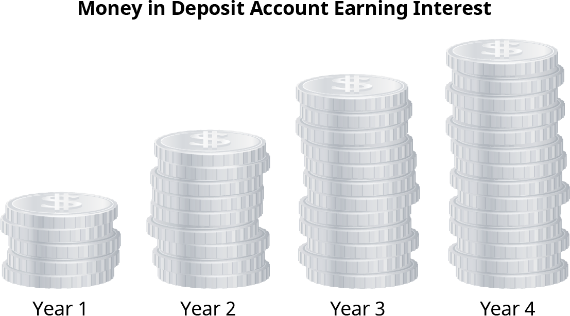
Figure 7.2 The Time Value of Money It is better to be paid today, or you will lose out on the money you would have earned in interest.

The Lump Sum Payment or Receipt

The most basic type of financial transaction involves a simple, one-time amount of cash, which can be either a receipt (inflow) or a payment (outflow). Such a one-time transaction is typically referred to as a lump sum. A lump sum consists of a one-off cash flow that occurs at any single point in time, present or future. Because it is always possible to dissect more complex transactions into smaller parts, the lump sum cash flow is the basis on which all other types of cash flow are treated. According to the general principle of adding value, every type of cash flow stream can be divided into a series of lump sums. For this reason, it is critical to understand the math associated with lump sums if you wish to have a greater appreciation, and a complete understanding, of more complicated forms of cash flow that may be associated with an investment or a capital purchase by a

company.

7.2
Time Value of Money (TVM) Basics

Learning Outcomes

By the end of this section, you will be able to:

• Define future value and provide examples.
• Explain how future dollar amounts are calculated using a single-period scenario.
• Describe the impact of compounding.

Because we can invest our money in interest-bearing accounts and investments, its value can grow over time as interest income accrues or returns are realized on our investments. This concept is referred to as future value (FV). In short, future value refers to how a specific amount of money today can have greater value tomorrow.

Single-Period Scenario

Let us start with the following example. Your friend is considering putting money in a bank account that will pay 4% interest per year and is particularly interested in knowing how much money they will have one year from now if they deposit $1,000 in this account. Your friend understands that you are studying finance and turns to you for help. By using the TVM principle of future value (FV), you can tell your friend that the answer is

$1,040. The additional $40 that will be in the account after one year will be due to interest earned over that time. You can calculate this amount relatively easily by taking the original deposit (also referred to as the principal) of $1,000 and multiplying it by the annual interest rate of 4% for one period (in this case, one year).

By taking the interest earned amount of $40 and adding it to the original principal of $1,000, you will arrive at a total value of $1,040 in the bank account at the end of the year. So, the $1,040 one year from today is equal to

$1,000 today when working with a 4% earning rate. Therefore, based on the concept of TVM, we can say that

$1,040 represents the future value of $1,000 one year from today and at a 4% rate of interest. We will discuss interest rates and their importance in TVM decisions in more detail later in this chapter; for now, we can consider interest rate as a percentage of the principal amount that is earned by the original lender of funds and/or charged to the borrower of these same funds. Following are a few more examples of the single-period scenario.

If a person deposits $300 in an account that pays 5% per year, at the end of one year, they will have

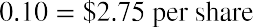
If a company has earnings of $2.50 per share and experiences a 10% increase in the following year, the earnings per share in year two are

If a retail store decides on a 3% price increase for the following year on an item that is currently selling for $50, the new price in the following year will be

The Impact of Compounding

What would happen if your friend were willing to wait one more year to receive their lump sum payment? What would the future dollar value in their account be after a two-year period? Returning to our earlier example, assume that during the second year, your friend leaves the principal ($1,000) and the earned interest ($40) in the account, thereby reinvesting the entire account balance for another year. The quoted interest rate of 4% reflects the interest the account would earn each year, not over the entire two-year savings period. So, during the second year of savings, the $1,000 deposit and the $40 interest earned during the first year would

both earn 4%:

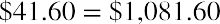
The additional $1.60 is interest on the first year’s interest and reflects the compounding of interest. Compound interest is the term we use to refer to interest income earned in subsequent periods that is based on interest income earned in prior periods. To put it simply, compound interest refers to interest that is earned on interest. Here, it refers to the $1.60 of interest earned in the second year on the $40.00 of interest earned in the first year. Therefore, at the end of two years, the account would have a total value of $1,081.60. This consists of the original principal of $1,000 plus the $40.00 interest income earned in year one and the $41.60 interest income earned in year two.

The amount of money your friend would have in the account at the end of two years, $1,081.60, is referred to as the future value of the original $1,000 amount deposited today in an account that will earn 4% interest every year.

Simple interest applies to year 1 while compound interest or “interest on interest” applies to year 2. This is calculated using the following method:

So, the total amount that would be in the account after two years, at 4% annual interest, would be

.

To determine any future value of money in an interest-bearing account, we multiply the principal amount by 1 plus the interest rate for each year the money remains in the account. From this, we can develop the future value formula:

In this formula, the number of times we multiply by depends entirely on the number of years the money will remain in the bank account, earning interest, before it is withdrawn in a final lump sum distribution paid out from the account at the end of the chosen savings period. The 1 in the formula represents the principal amount, or the original $1,000 deposit, which will be included in the final total lump sum payment when the account is closed and all money is withdrawn at the end of the predetermined savings period.

We can write the above equation in a more condensed mathematical form using time value of money notation, as follows:

Using these inputs, we have the following formula:

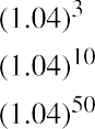
With this equation, we can calculate the value of the savings account after any number of years. For example, suppose we are considering 3, 10, and 50 years from the original deposit date at the annual 4% interest rate:

How can this savings account have grown to be so large after 50 years? This question is answered by the impact of compounding interest. Every year, the interest earned in previous years will also earn interest along

with the initial deposit. This will have the effect of accelerating the growth of the total dollar value of the account.

This is the important effect of the compounding of interest: money grows in larger and larger increments the longer you leave it in an interest-bearing account. In effect, the compounding of interest over time accelerates the growth of money.

In order to determine the FV of any amount of money, it will always be necessary to know the following pieces of information: (1) the principal, initial deposit, or present value (PV); (2) the rate of interest, usually expressed on an annual basis as r; and (3) the number of time periods that the money will remain in the account (n). The interest rate is often referred to as the growth rate, or the annual percentage increase on savings or on an investment. When the rate is raised to the power of the number of periods, the formula

will yield a number that is commonly referred to as the future value interest factor (FVIF). As a result of this process, as n (time, or the number of periods) increases, the future value interest factor will increase. Also, as r (interest rate) increases, the FVIF will increases. For these reasons, the future value calculation is directly determined by both the interest rate being used and the total amount of time—specifically, the number of periods—being considered.

THINK IT THROUGHCalculating Future ValuesHere’s another example of calculating future values in multiple-period scenarios.On a recent drive, you spotted your dream home, which is currently listed at $400,000. Unfortunately, you are not in a position to buy it right away and will have to wait at least another six years before you can afford it. If house values are appreciating at an annual rate of inflation of 4%, how much will a similar house cost after six years?Solution:In this case, PV is the current cost of the house, or $400,000; n is six years; r is the average annual inflation rate, or 4%; and we have to solve for FV.Therefore, under these circumstances, the house will cost $506,127.60 after six years.

How Time Impacts Compounding

We have just seen that time will lead to the growth of our money. As long as the prevailing growth or interest rate of any account we have our money in is positive, the passage of time will have the effect of growing the value of our money. The longer the period of time, the greater the growth and the larger the future value of the money will be. This can be reinforced very clearly with the following example.

Melvin is saving money in an account at a local bank that earns 5% per year. He begins with a deposit in his account of $100 and decides to save his money for exactly one year. He will not be making any further deposits into the account during the year. Melvin will earnor $5, in interest income. Adding this to the original deposit balance of $100 will give him a total of or $105, in the account at the end of one year.

Melvin likes this idea and believes he may be able to keep his money in the account for a longer period of time. How much money will he have in his account, without any further deposits, at the end of years two, three, four, and five?

Using the future value formula, the calculation is as follows:

How the Interest Rate Impacts Compounding

Melvin likes the idea of earning more money over time, but he also believes that what he would earn in interest may not be enough for some of the things he plans to buy in the future. His friend suggests finding an account or some form of investment with a greater interest rate than the 5% he can get at his local bank.

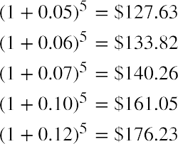Melvin thinks he can leave his money in an account or investment for a total of five years. He found investments that will provide annual returns of 6%, 7%, 10%, and 12%. Using the formula, we can complete the following calculations for him:

Again, Melvin likes this information, and he states that he will try to find the highest interest rate available. This makes sense, but it’s important to remember that investments are usually not guaranteed to earn you specific interest rates, or rates of return. Most investments, other than Treasury investments such as Treasury bonds, carry some form of financial risk, either small or large, and the greater the rate of return, the more likely it is that the risk associated with the investment will also be greater. This risk does not have any effect on the future calculations we have just completed, but it an important factor to bear in mind and consider well before moving ahead and putting your money in any investment or financial instrument.

7.3
Methods for Solving Time Value of Money Problems

Learning Outcomes

By the end of this section, you will be able to:

• Explain how future dollar amounts are calculated.
• Explain how present dollar amounts are calculated.
• Describe how discount rates are calculated.
• Describe how growth rates are calculated.
• Illustrate how periods of time for specified growth are calculated.
• Use a financial calculator and Excel to solve TVM problems.

We can determine future value by using any of four methods: (1) mathematical equations, (2) calculators with financial functions, (3) spreadsheets, and (4) FVIF tables. With the advent and wide acceptance and use of financial calculators and spreadsheet software, FVIF (and other such time value of money tables and factors) have become obsolete, and we will not discuss them in this text. Nevertheless, they are often still published in other finance textbooks and are also available on the internet to use if you so choose.

Using Timelines to Organize TVM Information

A useful tool for conceptualizing present value and future value problems is a timeline. A timeline is a visual,

linear representation of periods and cash flows over a set amount of time. Each timeline shows today at the left and a desired ending, or future point (maturity date), at the right.

Now, let us take an example of a future value problem that has a time frame of five years. Before we begin to solve for any answers, it would be a good approach to lay out a timeline like that shown in Table 7.1:

Year	0 (Today)	1	2	3	4	5

Table 7.1

The timeline provides a visual reference for us and puts the problem into perspective.

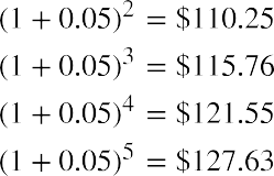
Now, let’s say that we are interested in knowing what today’s balance of $100 in our saving account, earning 5% annually, will be worth at the end of each of the next five years. Using the future value formula

that we covered earlier, we would arrive at the following values: $105 at the end of year one, $110.25 at the end of year two, $115.76 at the end of year three, $121.55 at the end of year four, and $127.63 at the end of year five.

With the numerical information, the timeline (at a 5% interest or growth rate) would look like Table 7.2:

Year	0	1	2	3	4	5
	$100.00	$105.00	$110.25	$115.76	$121.55	$127.63

Table 7.2

Using timelines to lay out TVM problems becomes more and more valuable as problems become more complex. You should get into the habit of using a timeline to set up these problems prior to using the equation, a calculator, or a spreadsheet to help minimize input errors. Now we will move on to the different methods available that will help you solve specific TVM problems. These are the financial calculator and the Excel spreadsheet.

Using a Financial Calculator to Solve TVM Problems

An extremely popular method of solving TVM problems is through the use of a financial calculator. Financial calculators such as the Texas Instruments BAII Plus™ Professional (https://openstax.org/r/baii-plus- professional) will typically have five keys that represent the critical variables used in most common TVM problems: N, I/Y, PV, FV, and PMT. These represent the following:

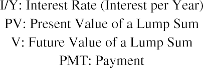
These are the only keys on a financial calculator that are necessary to solve TVM problems involving a single payment or lump sum.

Example 1: Future Value of a Single Payment or Lump Sum

Let’s start with a simple example that will provide you with most of the skills needed to perform TVM functions involving a single lump sum payment with a financial calculator.

Suppose that you have $1,000 and that you deposit this in a savings account earning 3% annually for a period of four years. You will naturally be interested in knowing how much money you will have in your account at the end of this four-year time period (assuming you make no other deposits and withdraw no cash).

To answer this question, you will need to work with factors of $1,000, the present value (PV); four periods or years, represented by N; and the 3% interest rate, or I/Y. Make sure that the calculator register information is cleared, or you may end up with numbers from previous uses that will interfere with the solution. The register- clearing process will depend on what type of calculator you are using, but for the TI BA II Plus™ Professional calculator, clearing can be accomplished by pressing the keys 2ND and FV [CLR TVM].

Once you have cleared any old data, you can enter the values in the appropriate key areas: 4 for N, 3 for I/Y, and 1000 for PV. Now you have entered enough information to calculate the future value. Continue by pressing the CPT (compute) key, followed by the FV key. The answer you end up with should be displayed as 1,125.51 (see Table 7.3).

Step123456DescriptionClear calculator registerEnterCE/CDisplayEnter present value (as a negative integer) 1000 +|- PV PV =Enter interest rate Enter time periodsIndicate no payments or depositsCompute future value3 I/Y4 N0 PMT CPT FVI/Y = N = PMT =FV =0.00-1,000.003.004.000.001,125.51

Table 7.3 Calculator Steps for Finding the Future Value of a Single Payment or Lump Sum¹

Important Notes for Using a Calculator and the Cash Flow Sign Convention

Please note that the PV was entered as negative $1,000 (or -$1000). This is because most financial calculators (and spreadsheets) follow something called the cash flow sign convention, which is a way for calculators and spreadsheets to keep the relative direction of the cash flow straight. Positive numbers are used to represent cash inflows, and negative numbers should always be used for cash outflows.

In this example, the $1,000 is an investment that requires a cash outflow. For this reason, -1000 is entered as the present value, as you will be essentially handing this $1,000 to a bank or to someone else to initiate the transaction. Conversely, the future value represents a cash inflow in four years’ time. This is why the calculator generates a positive 1,125.51 as the end result of this calculation.

Had you entered the present value of $1,000 as a positive number, there would have been no real concern, but the ending future value answer would have been returned expressed as a negative number. This would be correct had you borrowed $1,000 today (cash inflow) and agreed to repay $1,125.51 (cash outflow) four years from now. Also, it is important that you do not change the sign of any input value by using the – (minus) key). For example, on the TI BA II Plus™ Professional, you must use the +|- key instead of the minus key. If you enter 1000 and then hit the +|- key, you will get a negative 1,000 amount showing in the calculator display.

An important feature of most financial calculators is that it is possible to change any of the variables in a problem without needing to reenter all of the other data. For example, suppose that we wanted to find out the future value in our bank account if we left the money from our previous example invested for 20 years instead

1 The specific financial calculator in these examples is the Texas Instruments BA II Plus™ Professional model, but you can use other financial calculators for these types of calculations.

THINK IT THROUGHHow to Determine Future Value When Other Variables Are KnownHere’s an example of using a financial calculator to solve a common time value of money problem. You have $2,000 invested in a money market account that is expected to earn 4% annually. What will be the total value in the account after five years?Solution:Follow the recommended financial calculator steps in Table 7.4.Table 7.4 Calculator Steps for Determining Future ValueThe result of this future value calculation of the invested money is $2,433.31.
of 4. Before clearing any of the data, simply enter 20 for N and then press the CPT key and then the FV key. After this is done, all other inputs will remain the same, and you will arrive at an answer of $1,806.11.

Step	Description	Enter	Display
1	Clear calculator register	CE/C	0.00
2	Enter present value (as a negative integer)	2000 +|- PV	PV =-2,000.00
3	Enter interest rate	4 I/Y	I/Y =4.00
4	Enter time periods	5 N	N =5.00
5	Indicate no payments or deposits	0 PMT	PMT =0.00
6	Compute future value	CPT FV	FV =2,433.31

Example 2: Present Value of Lump Sums

Solving for the present value (discounted value) of a lump sum is the exact opposite of solving for a future value. Once again, if we enter a negative value for the FV, then the calculated PV will be a positive amount.

Taking the reverse of what we did in our example of future value above, we can enter -1,125.51 for FV, 3 for

I/Y, and 4 for N. Hit the CPT and PV keys in succession, and you should arrive at a displayed answer of 1,000.

An important constant within the time value of money framework is that the present value will always be less than the future value unless the interest rate is negative. It is important to keep this in mind because it can help you spot incorrect answers that may arise from errors with your input.

THINK IT THROUGHHow to Determine Present Value When Other Variables Are KnownHere is another example of using a financial calculator to solve a common time value of money problem. You have just won a second-prize lottery jackpot that will pay a single total lump sum of $50,000 five years from now. How much value would this have in today’s dollars, assuming a 5% interest rate?Solution:Follow the recommended financial calculator steps in Table 7.5.

Step123456DescriptionClear calculator registerEnterCE/CDisplayEnter future value (as a negative integer) 50000 +|- FV FV =Enter interest rate Enter time periodsIndicate no payments or depositsCompute present value5 I/Y5 N0 PMT CPT PVI/Y = N = PMT =PV =0.00-50,000.005.005.000.0039,176.31Table 7.5 Calculator Steps for Determining Present ValueThe present value of the lottery jackpot is $39,176.31.

Example 3: Calculating the Number of Periods

There will be times when you will know both the value of the money you have now and how much money you will need to have at some unknown point in the future. If you also know the interest rate your money will be earning for the foreseeable future, then you can solve for N, or the exact amount of time periods that it will take for the present value of your money to grow into the future value that you will require for your eventual use.

Now, suppose that you have $100 today and you would like to know how long it will take for you to be able to purchase a product that costs $133.82.

After making sure your calculator is clear, you will enter 5 for I/Y, -100 for PV, and 133.82 for FV. Now press

CPT N, and you will see that it will take 5.97 years for your money to grow to the desired amount of $133.82.

Again, an important thing to note when using a financial calculator to solve TVM problems is that you must enter your numbers according to the cash flow sign convention discussed above. If you do not make either the PV or the FV a negative number (with the other being a positive number), then you will end up getting an error message on the screen instead of the answer to the problem. The reason for this is that if both numbers you enter for the PV and FV are positive, the calculator will operate under the assumption that you are receiving a financial benefit without making any cash outlay as an initial investment. If you get such an error message in your calculations, you can simply press the CE/C key. This will clear the error, and you can reenter your data correctly by changing the sign of either PV or FV (but not both of these, of course).

THINK IT THROUGHDetermining Periods of TimeHere is an additional example of using a financial calculator to solve a common time value of money problem. You want to be able to contribute $25,000 to your child’s first year of college tuition and related expenses. You currently have $15,000 in a tuition savings account that is earning 6% interest every year. How long will it take for this account grow into the targeted amount of $25,000, assuming no additional deposits or withdrawals will be made?Solution:Table 7.6 shows the steps you will take.

Step123456DescriptionClear calculator registerEnterCE/CEnter present value (as a negative integer) 15000 +|- PV PV =Enter interest rate Enter future valueIndicate no payments or depositsCompute time periods6 I/Y25000 FV0 PMT CPT NI/Y =FV =Display0.0000-15,000.00006.000025,000.0000PMT =N =0.00008.7667Table 7.6 Calculator Steps for Determining Period of TimeThe result of this calculation is a time period of 8.7667 years for the account to reach the targeted amount.

Example 4: Solving for the Interest Rate

Solving for an interest rate is a common TVM problem that can be easily addressed with a financial calculator. Let’s return to our earlier example, but in this case, we know that we have $1,000 at the present time and that we will need to have a total of $1,125.51 four years from now. Let’s also say that the only way we can add to the current value of our savings is through interest income. We will not be able to make any further deposits in addition to our initial $1,000 account balance.

What interest rate should we be sure to get on our savings account in order to have a total savings account value of $1,125.51 four years from now?

Once again, clear the calculator, and then enter 4 for N, -1,000 for PV, and 1,125.51 for FV. Then, press the CPT and I/Y keys and you will find that you need to earn an average 3% interest per year in order to grow your savings balance to the desired amount of $1,125.51. Again, if you end up with an error message, you probably failed to follow the sign convention relating to cash inflow and outflow that we discussed earlier. To correct this, you will need to clear the calculator and reenter the information correctly.

After you believe you are done and have arrived at a final answer, always make sure you give it a quick review. You can ask yourself questions such as “Does this make any sense?” “How does this compare to other answers I have arrived at?” or “Is this logical based on everything I know about the scenario?” Knowing how to go about such a review will require you to understand the concepts you are attempting to apply and what you are trying to make the calculator do. Further, it is critical to understand the relationships among the different inputs and variables of the problem. If you do not fully understand these relationships, you may end up with an incorrect answer. In the end, it is important to realize that any calculator is simply a tool. It will only do what you direct it to do and has no idea what your objective is or what it is that you really wish to accomplish.

THINK IT THROUGHDetermining Interest or Growth RateHere is another example of using a financial calculator to solve a common time value of money problem. Let’s use a similar example to the one we used when calculating periods of time to determine an interest or growth rate. You still want to help your child with their first year of college tuition and related expenses.You also still have a starting amount of $15,000, but you have not yet decided on a savings plan to use.

Step	Description	Enter	Display
1	Clear calculator register	CE/C	0.0000
2	Enter present value (as a negative integer)	15000 +|- PV	PV =-15,000.0000
3	Enter time periods	8.5 N	N =8.5000
4	Enter future value	25000 FV	FV =25,000.0000
5	Indicate no payments or deposits	0 PMT	PMT =0.0000
6	Compute interest rate	CPT I/Y	I/Y =6.1940

Instead, the information you now have is that your child is just under 10 years old and will begin college at age 18. For simplicity’s sake, let’s say that you have eight and a half years before you will need to meet your total savings target of $25,000. What rate of interest will you need to grow your saved money from $15,000 to $25,000 in this time period, again with no other deposits or withdrawals?Solution:Follow the steps shown in Table 7.7.Table 7.7 Calculator Steps for Determining Interest RateThe result of this calculation is a necessary interest rate of 6.194%.
Using Excel to Solve TVM Problems

Excel spreadsheets can be excellent tools to use when solving time value of money problems. There are dozens of financial functions available in Excel, but a student who can use a few of these functions can solve almost any TVM problem. Special functions that relate to TVM calculations are as follows:

Future Value (FV) Present Value (PV)

Number of Periods (NPER) Interest Rate (RATE)

Excel also includes a function called Payment (PMT) that is used in calculations involving multiple payments or deposits (annuities). These will be covered in Time Value of Money II: Equal Multiple Payments.

Future Value (FV)

The Future Value function in Excel is also referred to as FV and can be used to calculate the value of a single lump sum amount carried to any point in the future. The FV function syntax is similar to that of the other four basic time-value functions and has the following inputs (referred to as arguments), similar to the functions listed above:

Rate: Interest Rate Nper: Number of Periods

Pmt: Payment PV: Present Value

Lump sum problems do not involve payments, so the value of Pmt in such calculations is 0. Another argument,

Type, refers to the timing of a payment and carries a default value of the end of the period, which is the most common timing (as opposed to the beginning of a period). This may be ignored in our current example, which means the default value of the end of the period will be used.

The spreadsheet in Figure 7.3 shows two examples of using the FV function in Excel to calculate the future value of $100 in five years at 5% interest.

In cell E1, the FV function references the values in cells B1 through B4 for each of the arguments. When a user begins to type a function into a spreadsheet, Excel provides helpful information in the form of on-screen tips showing the argument inputs that are required to complete the function. In our spreadsheet example, as the FV formula is being typed into cell E2, a banner showing the arguments necessary to complete the function appears directly below, hovering over cell E3.

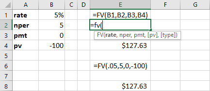
Figure 7.3 Using the FV Function in Excel

Cells E1 and E2 show how the FV function appears in the spreadsheet as it is typed in with the required arguments. Cell E4 shows the calculated answer for cell E1 after hitting the enter key. Once the enter key is pressed, the hint banner hovering over cell E3 will disappear. The second example of the FV function in our example spreadsheet is in cell E6. Here, the actual numerical values are used in the FV function equation rather than cell references. The method in cell E8 is referred to as hard coding. In general, it is preferable to use the cell reference method, as this allows for copying formulas and provides the user with increased flexibility in accounting for changes to input data. This ability to accept cell references in formulas is one of the greatest strengths of Excel as a spreadsheet tool.

Download the spreadsheet file (https://openstax.org/r/docs.google_uc_export) containing key Chapter 7 Excel exhibits.

Determining Future Value When Other Variables Are Known. You have $2,000 invested in a money market account that is expected to earn 4% annually. What will be the total value in the account in five years?

Note: Be sure to follow the sign conventions. In this case, the PV should be entered as a negative value.

Note: In Excel, interest and growth rates must be entered as percentages, not as whole integers. So, 4 percent must be entered as 4% or 0.04—not 4, as you would enter in a financial calculator.

Note: It is always assumed that if not specifically stated, the compounding period of any given interest rate is annual, or based on years.

Note: The Excel command used to calculate future value is as follows:

=FV(rate, nper, pmt, [pv], [type])

You may simply type the values for the arguments in the above formula. Another option is to use the Excel insert function option. If you decide on this second method, below are several screenshots of dialog boxes you will encounter and will be required to complete.

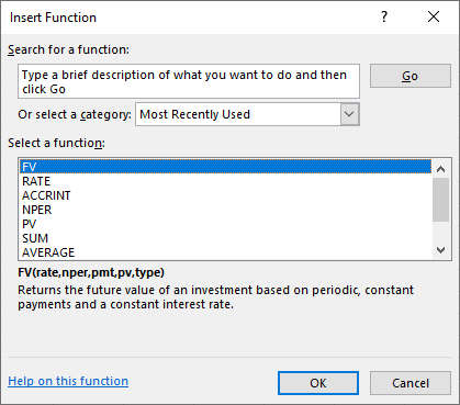• First, go to Formulas in the upper menu bar, and select the Insert Function option. When you do so, a dialog box will appear that looks like what you see in Figure 7.4.

Figure 7.4 Dialog Box to Insert FV Function

This dialog box allows you to either search for a function or select a function that has been used recently. In this example, you can search for FV by typing this in the search box and selecting Go, or you can simply choose FV from the list of most recently used functions (as shown here with the highlighted FV option).

• Once you select FV and click the OK button, a new dialog box will appear for you to enter the necessary details. See Figure 7.5.

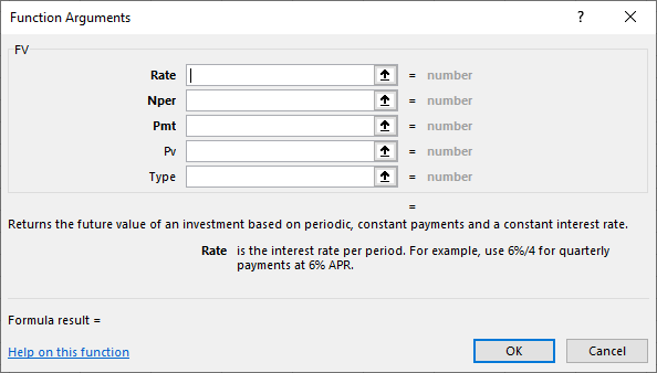
Figure 7.5 New Dialog Box for FV Function Arguments

Figure 7.6 shows the completed data input for the variables, referred to here as “function arguments.” Note that cell addresses are used in this example. This allows the spreadsheet to still be useful if you decide to change any of the variables. You may also type values directly into the Function Arguments dialog box, but if you do this and you have to change any of your inputs later, you will have to reenter the new information. Using cell addresses is always a preferable method of entering the function argument data.

Additional notes:

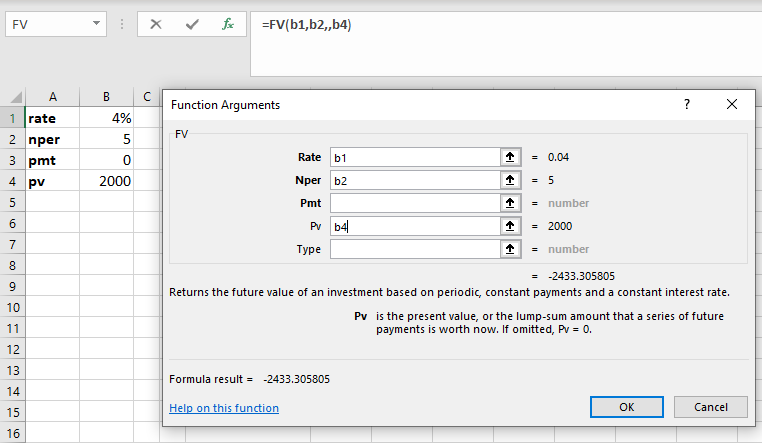
Figure 7.6 Completed Data Entry Menu for FV Function Arguments

• The Pmt argument or variable can be ignored in this instance, or you can enter a placeholder value of

zero. This example shows a blank or ignored entry, but either option may be used in problems such as this where the information is not relevant.

• The Type argument does not apply to this problem. Type refers to the timing of cash flows and is usually used in multiple payment or annuity problems to indicate whether payments or deposits are made at the beginning of periods or at the end. In single lump sum problems, this is not relevant information, and the Type argument box is left empty.
• When you use cell addresses as function argument inputs, the numerical values within the cells are displayed off to the right. This helps you ensure that you are identifying the correct cells in your function. The final answer generated by the function is also displayed for your preliminary review.

Once you are satisfied with the result, hit the OK button, and the dialog box will disappear, with only the final numerical result appearing in the cell where you have set up the function.

The FV of this present value has been calculated as approximately $2,433.31.

Present Value (PV)

We have covered the idea that present value is the opposite of future value. As an example, in the spreadsheet shown in Figure 7.3, we calculated that the future value of $100 five years from now at a 5% interest rate would be $127.63. By reversing this process, we can safely state that $127.63 received five years from now with a 5% interest (or discount) rate would have a value of just $100 today. Thus, $100 is its present value. In Excel, the PV function is used to determine present value (see Figure 7.7).

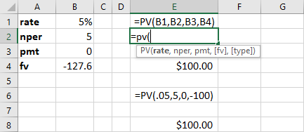
Figure 7.7 Using the PV Function in Excel

The formula in cell E1 uses cell references in a similar fashion to our FV example spreadsheet above. Also similar to our earlier example is the hard-coded formula for this calculation, which is shown in cell E6. In both cases, the answers we arrive at using the PV function are identical, but once again, using cell references is preferred over hard coding if possible.

THINK IT THROUGHDetermining Present Value When Other Variables Are KnownYou have just won a second-prize lottery jackpot that will pay a single total lump sum of $50,000 five years from now. You are interested in knowing how much value this would have in today’s dollars, assuming a 5% interest rate.

Notes:

• If you wish for the present value amount to be positive, the future value you enter here should be a negative value.
• In Excel, interest and growth rates must be entered as percentages, not as whole integers. So, 5 percent must be entered as 5% or 0.05—not 5, as you would enter in a financial calculator.
• It is always assumed that if not specifically stated, the compounding period of any given interest rate is annual, or based on years.
• The Excel command used to calculate present value is as shown here:

Solution:

=PV(rate, nper, pmt, [fv], [type])

As with the FV formula covered in the first tab of this workbook, you may simply type the values for the arguments in the above formula. Another option is to again use the Insert Function option in Excel. Figure 7.8, Figure 7.9, and Figure 7.10 provide several screenshots that demonstrate the steps you’ll need to follow if you decide to enter the PV function from the Insert Function menu.

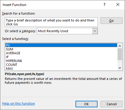• First, go to Formulas in the upper menu bar, and select Insert Function. When you do so, the Insert Function dialog box will appear (see Figure 7.8).

Figure 7.8 Dialog Box to Insert PV Function

As discussed in the FV function example above, this dialog box allows you to either search for a function or select a function that has been used recently. In this example, you can search for PV by typing this into the search box and selecting Go, or you can simply choose PV from the list of the most recently used functions.

• Once you have highlighted PV, click the OK button, and a new dialog box will appear for you to enter the necessary details. Similar to our FV function example, it will look like Figure 7.9.

Figure 7.9 New Dialog Box for PV Function Arguments

Figure 7.10 shows the completed data input for the function arguments. Note that once again, cell addresses are used in this example. This allows the spreadsheet to still be useful if you decide to change any of the variables. As in the FV function example, you may also type values directly in the Function Arguments dialog box, but if you do this and you have to change any of your input later, you will have to reenter the new information. Remember that using cell addresses is always a preferable method of entering the function argument data.

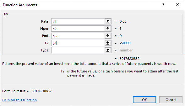
Figure 7.10 Completed Dialog Box for PV Function Arguments

Again, similar to our FV function example, the Function Arguments dialog box shows values off to the

right of the data entry area, including our final answer. The Pmt and Type boxes are again not relevant to this single lump sum example, for reasons we covered in the FV example.Review your answer. Once you are satisfied with the result, click the OK button, and the dialog box will disappear, with only the final numerical result appearing in the cell where you have set up the function. The PV of this future value has been calculated as approximately $39,176.31.

Periods of Time

The following discussion will show you how to use Excel to determine the amount of time a given present value will need to grow into a specified future value when the interest or growth rate is known.

You want to be able to contribute $25,000 to your child’s first year of college tuition and related expenses. You currently have $15,000 in a tuition savings account that is earning 6% interest every year. How long will it take for this account grow into the targeted amount of $25,000, assuming no additional deposits or withdrawals are made?

Notes:

• As with our other examples, interest and growth rates must be entered as percentages, not as whole integers. So, 6 percent must be entered as 6% or 0.06—not 6, as you would enter in a financial calculator.
• The present value needs to be entered as a negative value in accordance with the sign convention covered earlier.
• The Excel command used to calculate the amount of time, or number of periods, is this:

=NPER (rate, pmt, pv, [fv], [type])

As with our FV and PV examples, you may simply type the values of the arguments in the above formula, or we can again use the Insert Function option in Excel. If you do so, you will need to work with the various dialog boxes after you select Insert Function.

• First, go to Formulas in the upper menu bar, and select the Insert Function option. When you do so, the Insert Function dialog box will appear (see Figure 7.11).

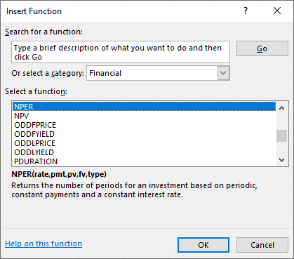
Figure 7.11 Dialog Box to Insert NPER Function

As discussed in our previous examples on FV and PV, this menu allows you to either search for a function or select a function that has been used recently. In this example, you can search for NPER by typing this into the search box and selecting Go, or you can simply choose NPER from the list of most recently used functions.

• Once you have highlighted NPER, click the OK button, and a new dialog box will appear for you to enter the necessary details. As in our previous examples, it will look like Figure 7.12.

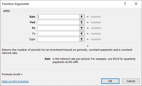
Figure 7.12 New Dialog Box for NPER Function Arguments

Figure 7.13 shows the completed Function Arguments dialog box. Note that once again, we are using cell addresses in this example.

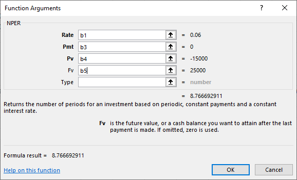
Figure 7.13 Completed Dialog Box for NPER Function Arguments

As in the previous function examples, values are shown off to the right of the data input area, and our final answer of approximately 8.77 is displayed at the bottom. Also, once again, the Pmt and Type boxes are not relevant to this single lump sum example.

Review your answer, and once you are satisfied with the result, click the OK button. The dialog box will disappear, with only the final numerical result appearing in the cell where you have set up the function.

The amount of time required for the desired growth to occur is calculated as approximately 8.77 years.

Interest or Growth Rate

You can also use Excel to determine the required growth rate when the present value, future value, and total number of required periods are known.

Let’s discuss a similar example to the one we used to calculate periods of time. You still want to help your child with their first year of college tuition and related expenses, and you still have a starting amount of $15,000, but you have not yet decided which savings plan to use.

Instead, the information you now have is that your child is just under 10 years old and will begin college at age

18. For simplicity’s sake, let’s say that you have eight and a half years until you will need to meet your total savings target of $25,000. What rate of interest will you need to grow your saved money from $15,000 to

$25,000 in this time, again with no other deposits or withdrawals?

Note: The present value needs to be entered as a negative value.

Interest Rate (RATE)

Note: The Excel command used to calculate interest or growth rate is as follows:

=RATE(nper, pmt, pv, [fv], [type], [guess])

As with our other TVM function examples, you may simply type the values for the arguments into the above formula. We also again have the same alternative to use the Insert Function option in Excel. If you choose this option, you will again see the Insert Function dialog box after you click the Insert Function button.

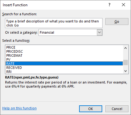• First, go to Formulas in the upper menu bar, and select the Insert Function option. When you do so, the Insert Function dialog box will appear (see Figure 7.14).

Figure 7.14 Dialog Box to Insert RATE Function

• This time, find and highlight RATE, and click the OK button once you have done so. The Function Arguments dialog box will look like Figure 7.15.

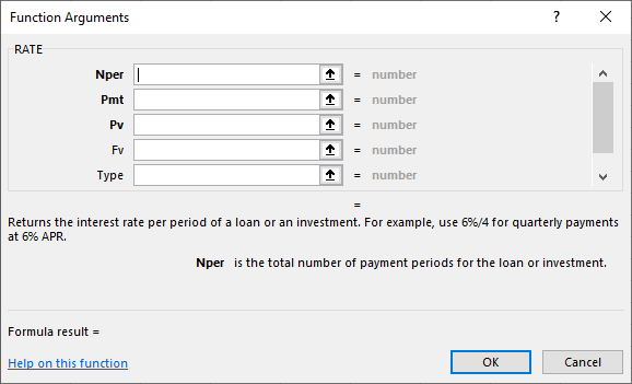
Figure 7.15 New Dialog Box for RATE Function Arguments

Once we complete the input, again using cell addresses for the required argument values, we will see what is shown in Figure 7.16.

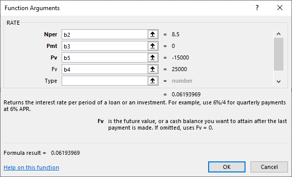
Figure 7.16 Completed Dialog Box for RATE Function Arguments

As in our other examples, cell values are shown as numerical values off to the right, and our answer of approximately 0.0619, or 6.19%, is shown at the bottom of the dialog box.

This answer also can be checked from a logic point of view because of the similar example we worked through when calculating periods of time. Our present value and future value are the same as in that example, and our time period is now 8.5 years, which is just under the result we arrived at (8.77 years) in

the periods example.

So, if we are now working with a slightly shorter time frame for the savings to grow from $15,000 into

$25,000, then we would expect to have a slightly greater growth rate. That is exactly how the answer turns out, as the calculated required interest rate of approximately 6.19% is just slightly greater than the growth rate of 6% used in the previous example. So, based on this, it looks like our answer here passes a simple “sanity check” review.

7.4
Applications of TVM in Finance

Learning Outcomes

By the end of this section, you will be able to:

• Explain how the time value of money can impact your personal financial goals.
• Explain how the time value of money is related to inflation.
• Explain how the time value of money is related to financial risk.
• Explain how compounding period frequency affects the time value of money.

Single-Period Scenario

Let’s say you want to buy a new car next year, and the one you have your eye on should be selling for $20,000 a year from now. How much will you need to put away today at 5% interest to have $20,000 a year from now? Essentially, you are trying to determine how much $20,000 one year from now is worth today at 5% interest over the year. To find a present value, we reverse the growth concept and lower or discount the future value back to the current period.

The interest rate that we use to determine the present value of a future cash flow is referred to as the discount rate because it is bringing the money back in time in terms of its value. The discount rate refers to the annual rate of reduction on a future value and is the inverse of the growth rate. Once we know this discount rate, we can solve for the present value (PV), the value today of tomorrow’s cash flow. By changing the FV equation, we can turn

into

which is the present value equation. The fraction shown above is referred to as the present value interest factor (PVIF). The PVIF is simply the reciprocal of the FVIF, which makes sense because these factors are doing exactly opposite things. Therefore, the amount you need to deposit today to earn $20,000 in one year at 5% interest is

The Multiple-Period Scenario

There will often be situations when you need to determine the present value of a cash flow that is scheduled to occur several years in the future (see Figure 7.17). We can again use the formula for present value to calculate a value today of future cash flows over multiple time periods.

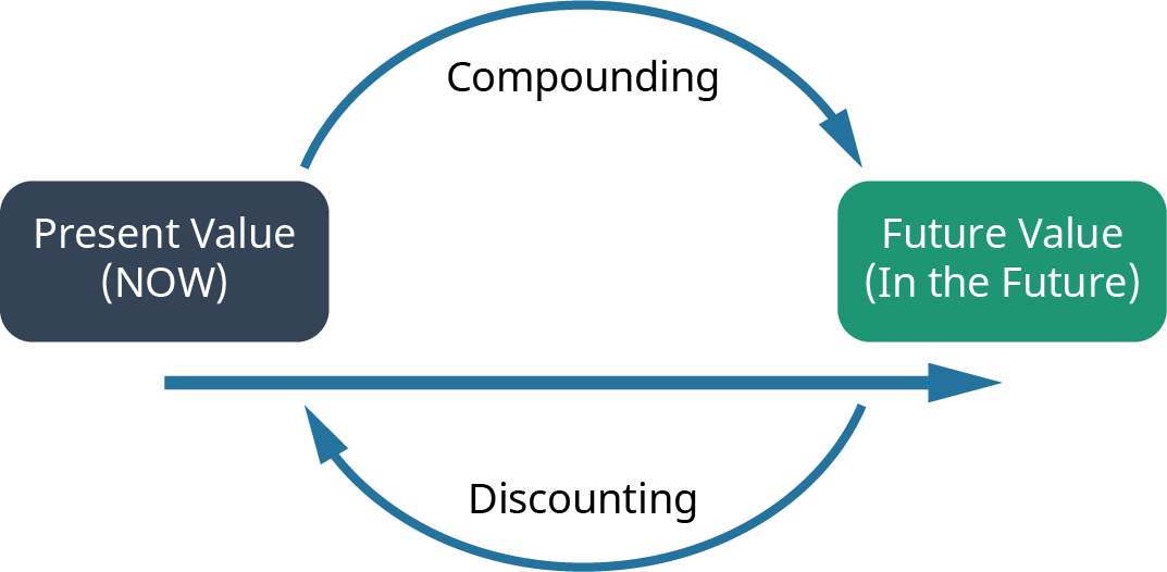
Figure 7.17 Determining Future Cash Flow

An example of this would be if you wanted to buy a savings bond for Charlotte, the daughter of a close friend. The face value of the savings bond you have in mind is $1,000, which is the amount Charlotte would receive in 30 years (the future value). If the government is currently paying 5% per year on savings bonds, how much will it cost you today to buy this savings bond?

The $1,000 face value of the bond is the future value, and the number of years n that Charlotte must wait to get this face value is 30 years. The interest rate r is 5.0% and is the discount rate for the savings bond. Applying the present value equation, we calculate the current price of this savings bond as follows:

So, it would cost you $231.38 to purchase this 30-year, 5%, $1,000 face-valued bond.

What we have done in the above example is reduce, or discount, the future value of the bond to arrive at a value expressed in today’s dollars. Effectively, this discounting process is the exact opposite of compounding interest that we covered earlier in our discussion of future value.

An important concept to remember is that compounding is the process that takes a present valuation of money to some point in the future, while discounting takes a future value of money and equates it to present dollar value terms.

Common applications in which you might use the present value formula include determining how much money you would need to invest in an interest-bearing account today in order to finance a college education for your oldest child and how much you would need to invest today to meet your retirement plans 30 years from now.

TVM, Inflation, Compounding Interest, Investing, Opportunity Costs, and Risk

The time value of money (TVM) is a critical concept in understanding the value of money relative to the amount of time it is held, saved, or invested. The TVM concept and its specific applications are frequently used by individuals and organizations that might wish to better understand the values of financial assets and to improve investing and saving strategies, whether these are personal or within business environments.

As we have discussed, the key element behind the concept of TVM is that a given amount of money is worth more today than that same amount of money will be at any point in the future. Again, this is because money can be saved or invested in interest-bearing accounts or investments that will generate interest income over time, thus resulting in increased savings and dollar values as time passes.

Inflation

The entire concept of TVM exists largely due to the presence of inflation. Inflation is defined as a general increase in the prices of goods and services and/or a drop in the value of money and its purchasing power.

The purchasing power of the consumer dollar is a statistic tracked by the part of the US Bureau of Labor

Statistics and is part of the consumer price index (CPI) data that is periodically published by that government agency. In a way, purchasing power can be viewed as a mirror image or exact opposite of inflation or increases in consumer prices, as measured by the CPI. Figure 7.18 demonstrates the decline in the purchasing power of the consumer dollar over the 13-year period from 2007 to 2020.

With this in mind, we can work with the TVM formula and use it to help determine the present value of money you have in hand today, as well as how this same amount of money may be valued at any specific point in the future and at any specific rate of interest.

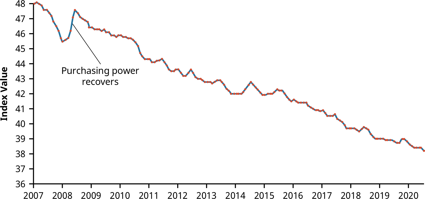
Figure 7.18 Historical Purchasing Power Decline as a Result of Inflation, 2007–2020 (data source: Bureau of Labor Statistics)

The Relationship between TVM and Inflation

As we have seen, the future value formula can be very helpful in calculating the value of a sum of cash (or any liquid asset) at some future point in time. One of the important ideas relating to the concept of TVM is that it is preferable to spend money today instead of at some point in the future (all other things being equal) when inflation is positive. However, in very rare instances in our economy when inflation is negative, spending money later is preferable to spending it now. This is because in cases of negative inflation, the purchasing power of a dollar is actually greater in the future, as the costs of goods and services are declining as we move into the future.

Most investors would be inclined to take a payment of money today rather than wait five years to receive a payment in the same amount. This is because inflation is almost always positive, which means that general prices of goods and services tend to increase over the passage of time. This is a direct function and result of normal economic growth. The crux of the concept of TVM is directly related to maintaining the present value of financial assets or increasing the value of these financial assets at different points in the future when they may be needed to obtain goods and services. If a consumer’s monetary assets grow at a greater rate than inflation over any period of time, then the consumer will realize an increase in their overall purchasing power. Conversely, if inflation exceeds savings or investment growth, then the consumer will lose purchasing power as time goes by under such conditions.

The Impact of Inflation on TVM

The difference between present and future values of money can be easily seen when considered under the effects of inflation. As we discussed above, inflation is defined as a state of continuously rising prices for goods and services within an economy. In the study of economics, the laws of supply and demand state that increasing the amount of money within an economy without increasing the amount of goods and services available will give consumers and businesses more money to spend on those goods and services. When more money is created and made available to the consuming public, the value of each unit of currency will diminish.

This will then have the effect of incentivizing consumers to spend their money now, or in the very near future, instead of saving cash for later use. Another concept in economics states that this relationship between money supply and monetary value is one of the primary reasons why the Federal Reserve might at times take steps to inject money into a stagnant, lethargic economy. Increasing the money supply will lead to increased economic activity and consumer spending, but it can also have the negative effect of increasing the costs of goods and services, furthering an increase in the rate of inflation.

Consumers who decide to save their money now and for the foreseeable future, as opposed to spending it now, are simply making the economic choice to have their cash on hand and available. So, this ends up being a decision that is made despite the risk of potential inflation and perhaps losing purchasing power. When inflationary risk is low, most people will save their money to have it available to spend later. Conversely, in times when inflationary risk is high, people are more likely to spend their money now, before its purchasing power erodes. This idea of inflationary risk is the primary reason why savers and investors who decide to save now in order to have their money available at some point in the future will insist they are paid, through interest or return on investment, for the future value of any savings or financial instrument.

Lower interest rates will usually lead to higher inflation. This is because, in a way, interest rates can be viewed as the cost of money. This allows for the idea that interest rates can be further viewed as a tax on holding on to sums of money instead of using it. If an economy is experiencing lower interest rates, this will make money less expensive to hold, thus incentivizing consumers to spend their money more frequently on the goods and services they may require. We have also seen that the more quickly inflation rates rise, the more quickly the general purchasing power of money will be eroded. Rational investors who set money aside for the future will demand higher interest rates to compensate them for such periods of inflation. However, investors who save for future consumption but leave their money uninvested or underinvested in low-interest-bearing accounts will essentially lose value from their financial assets because each of their future dollars will be worth less, carrying less purchasing power when they end up needing it for use. This relationship of saving and planning for the future is one of the most important reasons to understand the concept of the time value of money.

Nominal versus Real Interest Rates

One of the main problems of allowing inflation to determine interest rates is that current interest rates are actually nominal interest rates. Nominal rates are “stated,” not adjusted for the effects of inflation. In order to determine more practical real interest rates, the original nominal rate must be adjusted using an inflation rate, such as those that are calculated and published by the Bureau of Labor Statistics within the consumer price index (CPI).

A concept referred to as the Fisher effect, named for economist Irving Fisher, describes the relationship between inflation and the nominal and real interest rates and is expressed using the following formula:

where i is the nominal interest rate, R is the real interest rate, and h is the expected inflation rate.

An example of the Fisher effect would be seen in the case of a bond investor who is expecting a real interest rate of return of 6% on the bond, in an economy that is experiencing an expected inflation rate of 2%. Using the above formula, we have

So, the nominal interest rate on the bond amounts to 8.12%, with a real interest rate of 6% within an economy that is experiencing a 2% inflation rate. This is a logical result because in a scenario of positive inflation, a real rate of return would always be expected to amount to less than the stated or nominal rate.

Interest and Savings

Savings are adversely affected by negative real interest rates. A person who holds money in the form of cash is actually losing future purchasing value when real interest rates are negative. A saver who decides to hold

$1,000 in the form of cash for one year at a negative real interest rate of −3.65% per year will lose or $36.50, in purchasing power by the end of that year.

Ordinarily, interest rates would rise to compensate for negative real rates, but this might not happen if the Federal Reserve takes steps to maintain low interest rates to help stimulate and stabilize the economy. When interest rates are at such low levels, investors are forced out of Treasury and money market investments due to their extremely poor returns.

It soon becomes obvious that the time value of money is a critical concept because of its tremendous and direct impact on the daily spending, saving, and investment decisions of the people in our society. It is therefore extremely important that we understand how TVM and government fiscal policy can affect our savings, investments, purchasing behavior, and our overall personal financial health.

Compounding Interest

As we discussed earlier, compound interest can be defined as interest that is being earned on interest. In cases of compounding interest, the amount of money that is being accrued on previous amounts of earned interest income will continue to grow with each compounding period. So, for example, if you have $1,000 in a savings account and it is earning interest at a 10% annual rate and is compounded every year for a period of five years, the compounding will allow for growth after one year to an amount of $1,100. This comprises the original principal of $1,000 plus $100 in interest. In year two, you would actually be earning interest on the total amount from the previous compounding period—the $1,100 amount.

So, to continue with this example, by the end of year two, you would have earned $1,210 ($1,100 plus $110 in interest). If you continue on until the end of year five, that $1,000 will have grown to approximately $1,610. Now, if we consider that the highest annual inflation rate over the last 20 years has been 3%, then in this scenario, choosing to invest your present money in an account where interest is being compounded leaves you in a much better position than you would be in if you did not invest your money at all. The concept of the time value of money puts this entire idea into context for us, leading to more informed decisions on personal saving and investing.

It is important to understand that interest does not always compound annually, as assumed in the examples we have already covered. In some cases, interest can be compounded quarterly, monthly, daily, or even continuously. The general rule to apply is that the more frequent the compounding period, the greater the future value of a savings amount, a bond, or any other financial instrument. This is, of course, assuming that all other variables are constant.

The math for this remains the same, but it is important that you be careful with your treatment and usage of rate (r) and number of periods (n) in your calculations.

For example, $1,000 invested at 6% for a year compounded annually would be worth

. But that same $1,000 invested for that same period of time—one year—and earning interest at the same annual rate but compounded monthly would grow to

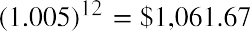, because the interest paid each month is earning interest on interest at a 6%

rate. Note that we represent r as the interest paid per period 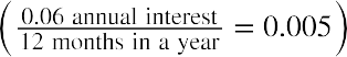and n as the number of periods (12 months in a year;) rather than the number of years, which is only one.

Continuing with our example, that same $1,000 in an account with interest compounded quarterly, or four times a year, would grow to 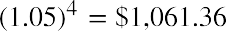in one year. Note that this final amount ends up being greater than the annually compounded future value of $1,060.00 and slightly less than the monthly

compounded future value of $1.061.67, which would appear to make logical sense.

The total differences in future values among annual, monthly, and quarterly compounding in these examples are insignificant, amounting to less than $1.70 in total. However, when working with larger amounts, higher interest rates, more frequent compounding periods, and longer terms, compounding periods and frequency become far more important and can generate some exceptionally large differences in future values.

Ten million dollars at 12% growth for one year and compounded annually amounts to

, while 10 million dollars on the same terms but compounded quarterly will

produce. Most wealthy and rational investors and savers would be very pleased to earn that additional $55,088.10 by simply having their funds in an account that features quarterly compounding.

In another example, $200 at 60% interest, compounded annually for six years, becomes

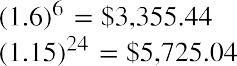, while this same amount compounded quarterly grows to

.

An amount of $1 at 3%, compounded annually for 100 years, will be worth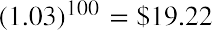. The same dollar at the same interest rate, compounded monthly over the course of a century, will grow to

.

This would all seem to make sense due to the fact that in situations when compounding increases in frequency, interest income is being received during the year as opposed to at the end of the year and thus grows more rapidly to become a larger and more valuable sum of money. This is important because we know through the concept of TVM that having money now is more useful to us than having that same amount of money at some later point in time.

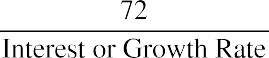
The Rule of 72

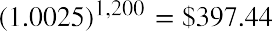
The rule of 72 is a simple and often very useful mathematical shortcut that can help you estimate the impact of any interest or growth rate and can be used in situations ranging from financial calculations to projections of population growth. The formula for the rule of 72 is expressed as the unknown (the required amount of time to double a value) calculated by taking the number 72 and dividing it by the known interest rate or growth rate. When using this formula, it is important to note that the rate should be expressed as a whole integer, not as a percentage. So, as a result, we have

This formula can be extremely practical when working with financial estimates or projections and for understanding how compound interest can have a dramatic effect on an original amount or monetary balance.

Following are just a few examples of how the rule of 72 can help you solve problems very quickly and very easily, often enabling you to solve them “in your head,” without the need for a calculator or spreadsheet.

Let’s say you are interested in knowing how long it will take your savings account balance to double. If your account earns an interest rate of 9%, your money will takeor 8, years to double. However, if you are earning only 6% on this same investment, your money will take, or 12, years to double.

Now let’s say you have a specific future purchasing need and you know that you will need to double your money in five years. In this case, you would be required to invest it at an interest rate of, or 14.4%. Through these sample examples, it is easy to see how relatively small changes in a growth or interest rate can have significant impact on the time required for a balance to double in size.

To further illustrate some uses of the rule of 72, let’s say we have a scenario in which we know that a country’s

gross domestic product is growing at 4% a year. By using the rule of 72 formula, we can determine that it will

take the economy 72/4, or 18, years to effectively double.

Now, if the economic growth slips to 2%, the economy will double in, or 36, years. However, if the rate of growth increases to 11%, the economy will effectively double in, or 6.55, years. By performing such calculations, it becomes obvious that reducing the time it takes to grow an economy, or increasing its rate of growth, could end up being very important to a population, given its current level of technological innovation and development.

It is also very easy to use the rule of 72 to express future costs being impacted by inflation or future savings amounts that are earning interest.

To apply another example, if the inflation rate in an economy were to increase from 2% to 3%, consumers would lose half of the purchasing power of their money. This is calculated as the value of their money doubling in, or 24, years as compared to, or 36, years—quite a substantial difference.

Now, let’s say that tuition costs at a certain college are increasing at a rate of 7% per year, which happens to be greater than current inflation rates. In this case, tuition costs would end up doubling in, or about 10.3, years.

In an example related to personal finance, we can say that if you happen to have an annual percentage rate of 24% interest on your credit card and you do not make any payments to reduce your balance, the total amount you owe to the credit card company will double in only , or 3, years.

So, as we have seen, the rule of 72 can clearly demonstrate how a relatively small difference of 1 percentage point in GDP growth or inflation rates can have significant effects on any short- or long-term economic forecasting models.

It is important to understand that the rule of 72 can be applied in any scenario where we have a quantity or an amount that is in the process of growing or is expected to grow for any period of time into the future. A good nonfinancial use of the rule of 72 might be to apply it to some population projections. For example, an increase in a country’s population growth rate from 2% to 3% could present a serious problem for the planning of facilities and infrastructure in that country. Instead of needing to double overall economic capacity inor 36, years, capacity would have to be expanded in only, or 24, years. It is easy to see how dramatic an effect this would be when we consider that the entire schedule for growth or infrastructure would be reduced by 12 years due to a simple and relatively small 1% increase in population growth.

Investing and Risk

Investing is usually a sound financial strategy if you have the money to do so. When investing, however, there are certain risks you should always consider first when applying the concepts of the time value of money. For example, making the decision to take $1,000 and invest it in your favorite company, even if it is expected to provide a 5% return each year, is not a guarantee that you will earn that return—or any return at all, for that matter. Instead, as with any investment, you will be accepting the risk of losing some or even all of your money in exchange for the opportunity to beat inflation and increase your future overall wealth. Essentially, it is risk and return that are responsible for the entire idea of the time value of money.

Risk and return are the factors that will cause a rational person to believe that a dollar risked should end up earning more than that single dollar.

To summarize, the concept of the time value of money and the related TVM formulas are extremely important because they can be used in different circumstances to help investors and savers understand the value of their money today relative to its earning potential in the future. TVM is critical to understanding the effect that inflation has on your money and why saving your money early can help increase the value of your savings dollars by giving them time to grow and outpace the effects of inflation.

Opportunity Costs

The concept of opportunity cost arises from the idea that there will always be possible options that are sacrificed with every option we decide on or for every choice that we make. For example, let’s consider the decision to go to college after you graduate from high school. This decision, as with just about any other, will involve evaluating opportunity costs. If you choose to go to college, this will result in your sacrificing four years of potential earnings that you could have had if you had decided to take a job instead of attending school.

Also, in addition to the lost salary, you would be losing out on four years of work experience that could have had a positive impact on your résumé or your future earnings prospects.

Of course, the entire idea behind furthering one’s education is that you are hopeful that by choosing to go to college, you will increase the likelihood of earning a greater salary over the course of your lifetime than you would have if you had chosen to join the workforce directly out of high school. So, this ends up being a bit of a risk, but one that you have considered. The idea is that you are hoping for a more significant payoff down the road than if you had made the decision not to continue with your studies. When it comes to opportunity costs and the time value of money, it is obvious that there will always be costs associated with every forgone financial opportunity we pass on when we make a different choice. The logical individual can only hope that these choices produce a better end result than if we had made different choices and pursued any of our forgone alternatives. This also applies in situations where we may sit idly by and decide to take no action at all.

For example, if you are putting $1,000 in a savings account to save for a house, you may be giving up an opportunity to grow that money in an investment account that would earn a greater rate of return. In another example, being able to calculate the future value of your money will tell you that instead of investing, you probably should be paying down your 24% APR credit card debt that is costing you hundreds of dollars a month—hundreds of dollars more than you might earn from an investment account.

Summary

Now versus Later Concepts

This section discussed the underlying concepts of the time value of money (TVM). Because it is possible to earn interest income on cash that you decide to deposit in an investment or an interest-bearing account, money that you have now or receive sooner will be more valuable to you than the same amount of money received later.

Time Value of Money (TVM) Basics

Future value refers to the value that a current amount will eventually grow into at a given interest rate over a specific period of time. The single-period scenario is one way in which future amounts are calculated.

Compounding, which is interest earned on interest, also affects the future value of money.

Methods for Solving Time Value of Money Problems

Calculations can be used to determine future and present dollar amounts, discount and growth rates, and periods of time required for specific growth. Time value of money problems can be solved using mathematical equations, calculators with financial functions, and spreadsheets. A useful tool for conceptualizing present value and future value problems is a timeline. A timeline is a visual, linear representation of the timing of periods and cash flows over a set amount of time.

Applications of TVM in Finance

The idea of the time value of money is often considered to be the cornerstone concept of the study of finance. TVM can help investors and savers understand the value of money today relative to its earning potential in the future. TVM is critical to understanding the effect that inflation has on money and why saving your money early can help increase the value of your savings dollars by giving them time to grow and outpace the effects of inflation. Of course, it is important to remember that there will always be possible options that are sacrificed with every option you decide on and every choice you make.

Key Terms

Bureau of Labor Statistics a group within the United States Department of Labor that is the primary fact- finding agency for the US government in the fields of labor, statistics, and economics; serves as the principal agency of the US Federal Statistical System

compounding interest the continual addition of interest to the original principal sum of a loan or deposit, often referred to as interest on interest

compounding period the period between points in time when interest is paid or added to the principal

consumer price index (CPI) a measure that examines the weighted average of prices of a basket of consumer goods and services such as transportation, food, and medical care

discount rate the interest rate used to determine the present value of future cash inflows

Federal Reserve the central bank system of the United States

financial instrument an asset or bundle of assets, including monetary contracts between parties, that can be bought, sold, or traded for financial gain

financial risk the possibility of losing money or purchasing power on an investment, business transaction, or venture or simply due to inflation

Fisher effect an economic theory created by economist Irving Fisher that describes the relationship between inflation and both real and nominal interest rates

future value (FV) the value that a current amount will grow to at a given interest rate over a given period of time

gross domestic product (GDP) the total value of goods produced and services provided in a country during one year

growth rate the percentage increase of a specific variable within a specific time period; synonymous with

interest rate in the context of the time value of money

interest the amount of money that is paid by a borrower to a lender for the use of their money, typically calculated from an annualized rate

investment an asset or item acquired with the goal of generating financial gain through increased income or appreciation in value

liquid asset an asset that can be readily converted into cash within a short period of time

money market investments low-risk financial instruments such as T-bills, federal notes, commercial paper, certificates of deposit (CDs), repurchase agreements (repos), and bankers’ acceptances, among others money supply the total dollar value of legal tender that is available to consumers within an economy at any

single point in time

opportunity cost the loss of potential gain from other alternatives when a single alternative is chosen

present value (PV) the current value of a future amount, calculated by discounting the future value back at a known discount or interest rate for a specified period of time

real interest rate a rate of interest that has been adjusted to account for the effects of inflation

single payment or lump sum a single payment or deposit made at one time, as opposed to a number of smaller payments or deposits made in installments

time value of money (TMV) the concept that an amount of money is worth more today than the exact same amount of money at some point in the future

Treasury investments debt obligations such as T-bills (Treasury bills), bonds, and notes issued by the US Department of the Treasury

underinvested describes an insufficient amount of investment or an investment that is earning an insufficient rate of interest

uninvested describes cash that is being held in reserve, is not invested in an account or financial instrument, and is not earning interest or any return