4 Lesson 2 a Financial Forecasting Cash Budgets

Though no one in business has a crystal ball, managers must often do all they can to predict the future as accurately as possible. This is called forecasting. Accounting and finance professionals use past performance along with what they know about the business, its competitors, the economy, and the company’s plans for the future to assemble detailed financial forecasts. Forecasts are useful to many individuals for different reasons. A budget, a type of static forecast, helps accountants and managers see how their plans for the coming year can be achieved. It outlines sales targets and how much can be spent on cost of goods sold and expenses to achieve the company’s bottom-line (net income) targets. Investors use financial forecasts to help guide their decisions to buy, sell or hold stocks or to estimate future potential income through dividends. Perhaps most importantly, for our purposes in finance, forecasts are used to help predict and manage cash flows.

A business can have all the profit in the world at the end of the year, but if it doesn’t raise enough cash (liquidity) to pay the bills and pay its employees halfway through the year, it could still go bankrupt despite being profitable. Forecasting sales and expenses helps assemble a cash forecast—when sales will be collected and when expenses will be paid—so that financial managers can look forward far enough to have enough time to react accordingly and secure short- or long-term financing to meet gaps in cash flow.

18.1
The Importance of Forecasting

Learning Outcomes

By the end of this section, you will be able to:

• Discuss how to use financial statements in forecasting firm financials.
• Explain why balance sheet items are important in forecasting a firm’s financial result.
• Explain why income statement items are important in forecasting a firm’s financial result.

In this section, we will briefly review some of the basic elements of financial statements and how we can analyze historical statements to help assemble financial forecasts. Financial forecasting is important to short- and long-term firm success. It helps a firm plan for the resources it will need, ensuring it will have enough cash on hand at the right time to cover daily operations and capital expenditures. It helps the firm communicate its future potential and manage its shareholders’ expectations. It also helps management assess future risk and set plans in place to mitigate that risk.

Financial forecasting involves using historical data, analysis tools, and other information we can gather to make an educated guess about the future financial performance of the firm. Historical figures provide a reasonable starting point. We use tools such as ratios, common size, and trend analysis to fine-tune our forecast. And finally, we assess what we know about the firm, its competitors, the economy, and anything else that might impact performance and further fine-tune our forecast from there.

It’s important to take a moment to consider the role of ethics in forecasting. Ethics is a huge issue in the world of accounting and finance in general, and forecasting is no different. There can be tremendous pressure on management to perform, to deliver certain levels of profit, and to meet shareholder expectations.

Forecasting, as you will learn throughout this chapter, is not an exact science. There is a great deal of subjectivity that can come into play when forecasting sales and expenses. Ethical behavior is crucial in this area. Those who create forecasts must have a firm understanding of where their data comes from, how reliable it is, and whether or not their assumptions and projections are reasonably justified.

Financial Statement Foundations

In Financial Statements, you were introduced to a firm called Clear Lake Sporting Goods. You learned about the four key financial statements: the income statement, balance sheet, statement of stockholders’ equity, and statement of cash flows. Each one provides a different view of the firm’s financial health and performance.

Clear Lake Sporting Goods is a small merchandising company (a company that buys finished goods and sells them to consumers) that sells hunting and fishing gear. It uses financial statements to understand its profitability and current financial position, to manage cash flow, and to communicate its finances to outside parties such as investors, governing bodies, and lenders. We will use Clear Lake’s company information and historical financial statements in this chapter as we explore its forecasting process. It’s important to note that in this chapter, we are focusing on just one firm and the one method its managers have chosen to forecast financial performance. There are a variety of types of firms in actual application, and they may choose to forecast their financial performance differently. We are demonstrating just one approach here.

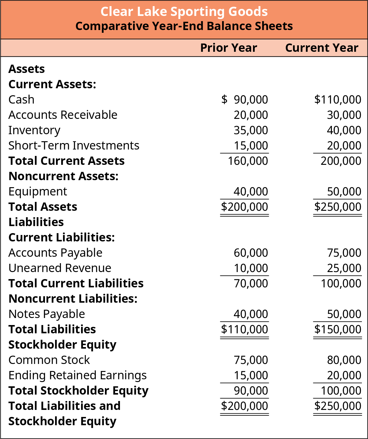
The balance sheet shows all the firm’s assets, liabilities, and equity at one point in time. It also supports the accounting equation in a very clear and transparent way. We find one section of the balance sheet contains all current and noncurrent assets that must total the other section of the balance sheet: total liabilities and equity. In Figure 18.2, we see that Clear Lake Sporting Goods has total assets of $250,000 in the current year, which balances with its total liabilities and equity of $250,000.

Figure 18.2 Balance Sheet

The income statement reflects the performance of the firm over a period of time. It includes net sales, cost of goods sold, operating expenses, and net income. In Figure 18.3, we see that Clear Lake had $120,000 in net sales, $60,000 in cost of goods sold, and $35,000 in net income in the current year.

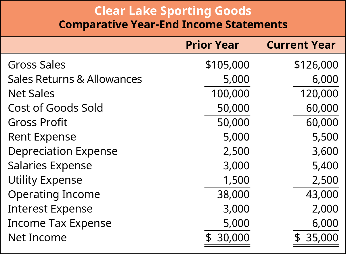
Figure 18.3 Full Income Statement

Finally, the statement of cash flows is used to reconcile net income to cash balances. The statement begins with net income, then reflects adjustments to balance sheet accounts and noncash expenses. The statement of

cash flows is broken down into three key categories: operating, investing, and financing. This allows users to clearly see what elements of the business are generating or using cash. In Figure 18.4, we see that Clear Lake had cash flow from operating activities of $53,600, cash used for investing activities of ($18,600), and cash used for financing activities of ($15,000).

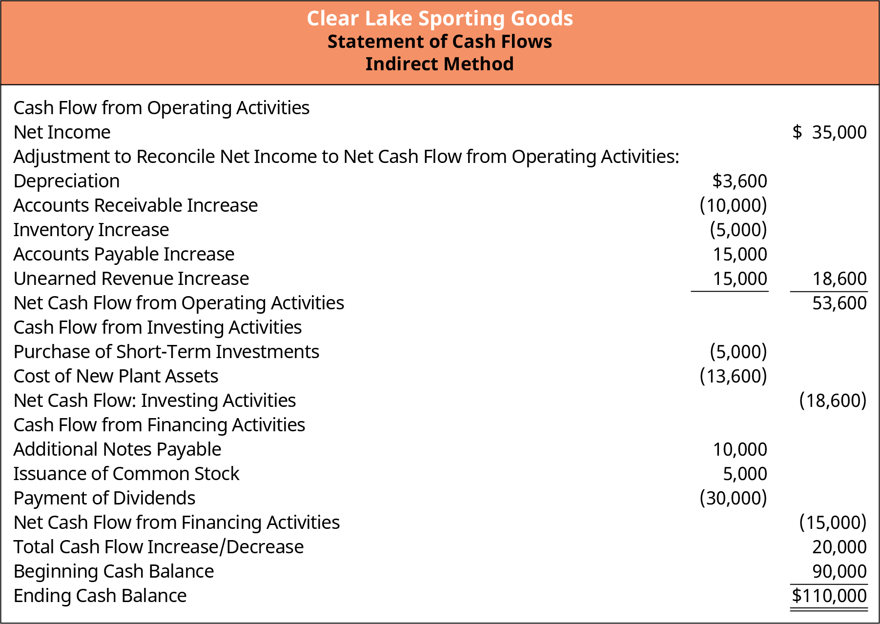
Figure 18.4 Statement of Cash Flows

Another key concept to remember about the financial statements is that the statement of cash flows is necessary to truly understand how the firm is using and generating cash. A common misconception is that if a firm reports net income on its income statement, then it must have plenty of cash, and if it reports a loss, it must be short on cash. Although this can be true, it’s not necessarily the case. Historically speaking, we need the statement of cash flows to get the full picture of how cash was used or generated in the past. Looking to the future, we need a cash flow forecast to plan for possible gaps in cash flow and, potentially, how to make the best use of any cash surplus. Throughout this chapter, we will see how to use historical financial statements to help develop the future cash forecast.

It’s also important to remember that the four financial statements are tied together. Net income from the income statement feeds into retained earnings, which live on the balance sheet. Equity balances on the balance sheet feed information to the statement of stockholders’ equity. And information from both the income statement (net income and noncash expenses) and the balance sheet (changes in working capital accounts) all feed into the statement of cash flows. These relationships will be helpful to understand when using historical statements and preparing forecasts.

Balance Sheet Analysis

Fully understanding the items that are on the balance sheet and how they relate to one another and to other financial statements will help you create a financial forecast. In Financial Statements, you learned that on the classified balance sheet, both assets and liabilities are broken down into current and noncurrent categories. You also know that the balance sheet must live up to its name—it must balance. This means that total assets (what the company owns) must equal total liabilities and equity (what the company owes).

You continued your financial statement development in Measures of Financial Health, where you saw how to use elements of the balance sheet to assess financial health. Ratios based on balance sheet accounts can be useful for understanding relationships between balance sheet items—how they related in the past and then, in forecasting, how those relationships might change or remain the same in the future. Examples of balance sheet ratios include the current ratio, quick ratio, cash ratio, debt-to-assets ratio, and debt-to-equity ratio.

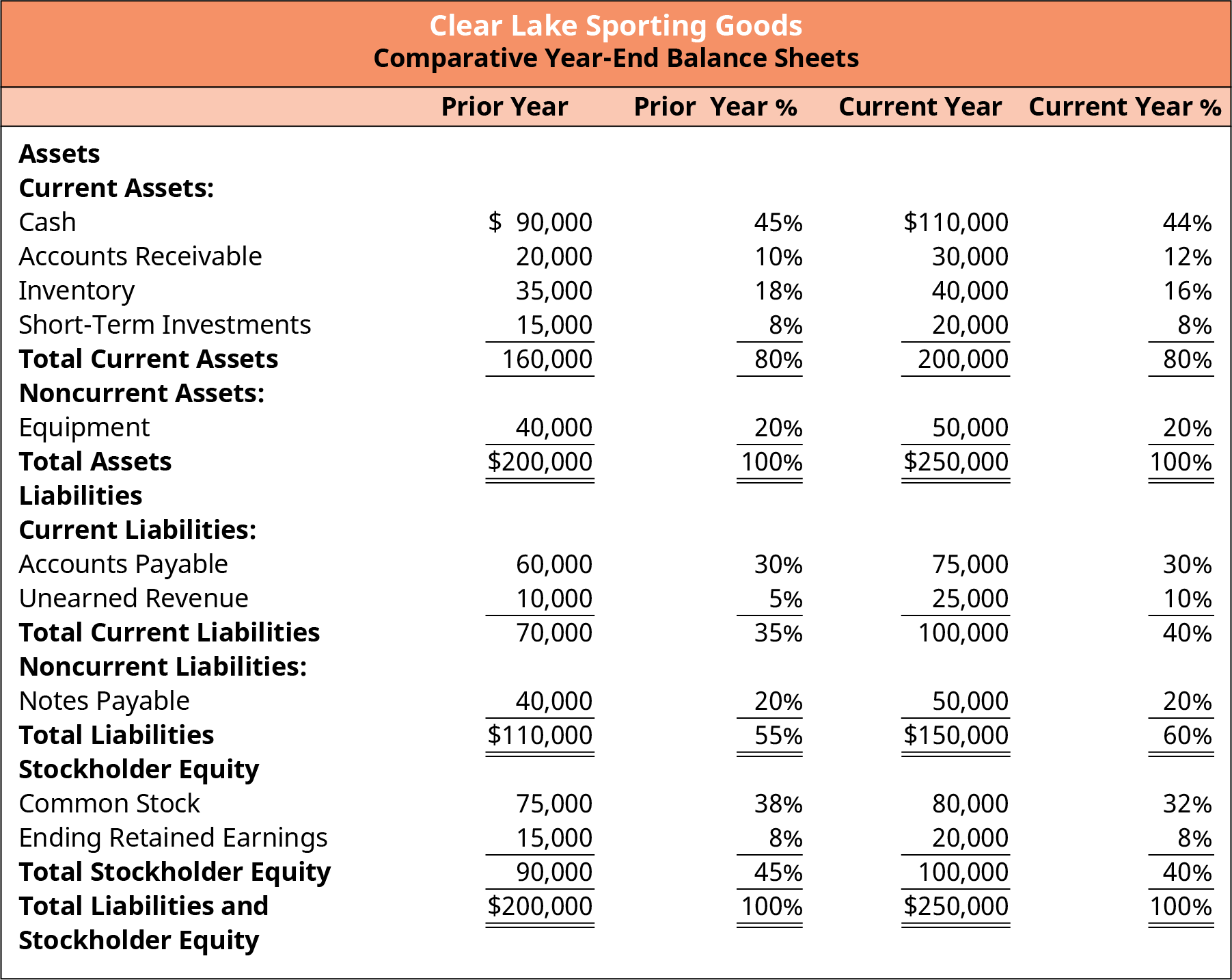
In Financial Statements, you also explored common-size analysis. To prepare a common-size analysis of the balance sheet, every item on the statement must be expressed as a percentage of total assets. Seeing each item as a percentage—that is, seeing its relationship to total assets—is also helpful for assessing historical statements and how those percentages or relationships can be used to predict future balances in the forecast. For example, in Figure 18.5, you can see that Clear Lake’s current assets represented 80% of its total assets in both the current and prior years.

Income Statement Analysis

Figure 18.5 Common-Size Balance Sheet

Like balance sheet analysis, income statement analysis is also quite helpful in preparing for the forecasting process. In Financial Statements, you learned that the income statement is commonly broken down into a few sections. Cost of goods sold is deducted from net sales to arrive at gross margin. Gross margin refers to the profits earned solely on the sale of the product itself, without consideration for the expenses incurred to run the business. Next, operating expenses are deducted to reflect operating income. Operating income reflects the profits of the core business function. Finally, other items, such as interest expense, tax expense, and other gains and losses, are deducted to arrive at net income, a.k.a. the bottom line. Each segment of the income statement is helpful for assessing past performance and estimating future expenses for a forecast.

You continued your financial statement development in Measures of Financial Health, where you saw how to

use elements of the income statement to assess historical financial performance. Ratios based on the income statement can be useful for understanding relationships between net sales and expenses—how they related in the past and then, in forecasting, how those relationships might change or remain the same. Examples of income statement ratios include gross margin, operating margin, and profit margin. Common ratios that incorporate items from both the balance sheet and the income statement include return on assets (ROA), return on equity (ROE), inventory turnover, accounts receivable turnover, and accounts payable turnover.

LINK TO LEARNINGPerformance TrendsReview the most recent annual report for Big 5 Sporting Goods (https://openstax.org/r/ annual_report_for_Big_5_Sporting-Goods). Review the company’s sales and gross margins for the current and past two years. How is their performance? Are their sales trending up or down? Why might the contribution margin have increased or decreased?

In Financial Statements, you also explored common-size analysis. To prepare a common-size analysis of the income statement, every item on the statement must be expressed as a percentage of net assets. Seeing each item as a percentage, in terms of its relationship to total sales, is also helpful for assessing historical statements and how those percentages or relationships can be used to predict future balances in the forecast. For example, in Figure 18.6, you can see that Clear Lake’s cost of goods sold represented 50% of its net sales in both the current and prior years.

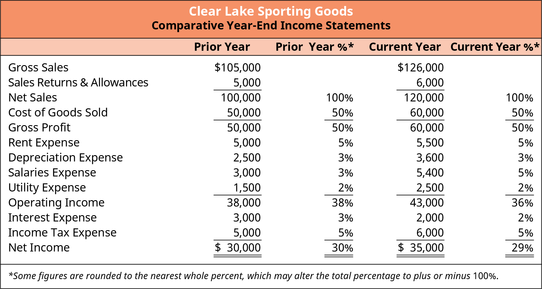
Figure 18.6 Common-Size Income Statement

18.2
Forecasting Sales

Learning Outcomes

By the end of this section, you will be able to:

• Explain how sales are the main driver for a financial forecast.
• Determine a past time period to formulate the basis for a financial forecast.
• Explain the advantages and disadvantages of using past data to forecast future financial performance.
• Calculate past sales growth averages.
• Justify adjusting relationships when forecasting future financial performance.

In this section of the chapter, you will begin to explore the first step of creating a forecast: forecasting sales. We will discuss common time frames for sales forecasts and why we use historical data in our forecasts (but only with caution), and we will work through the process of forecasting future sales. We will be using the percent-of-sales method to forecast some expenses for Clear Lake Sporting Goods, the example used throughout the chapter. This method relies on sales data, further highlighting why accuracy in forecasting sales is crucial.

Sales as the Driver

A significant portion of a business’s costs are driven by how much it sells. Thus, the sales forecast is the necessary first step in preparing a financial forecast. Common costs driven by sales include direct product costs, direct labor costs, and other key variable costs (i.e., costs that vary proportionately to sales), such as sales commissions.

Looking to the Past

Forecasting sales is not always an easy task, as no one knows the future. We can, however, use the information we do have to forecast future sales with the greatest accuracy possible. Most firms start by looking at the past. A firm may look at past sales from a variety of prior periods. It’s common to look at the past 12 months to estimate the coming 12 months. Looking at 12 consecutive months helps identify seasonality of sales trends, what time of year sales tend to drop off and when they increase, possible sales spikes that might reoccur, and any other trends that tend to appear over a 12-month period. In Figure 18.7, we see Clear Lake’s sales by month for the past 12 months.

Past data is often used in conjunction with probabilities and weighted average calculations derived from probabilities. Though used in several areas of forecasting, this approach is particularly common in drafting the sales forecast. Using multiple scenarios and the probability of each scenario occurring is a common approach to estimating future sales.

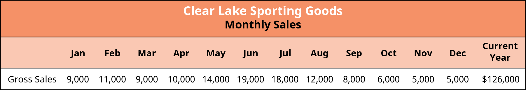
Figure 18.7 Historical Sales Data

We can see at first glance that sales remain fairly steady from January to April. Sales then goes up significantly in April and May, seem to peak in June, taper off a bit in July, then decline steeply from August to the end of the year, with the lowest sales being in November and December. Though not exact, it’s easy to quickly see that sales follow a seasonal pattern. We will focus on just one year of data here to keep things simple. However, it’s important to note that when a firm has a seasonal sales pattern, it normally uses more than one year of data to detect and evaluate the pattern. It’s not uncommon for firms to have a seasonal sales pattern that fluctuates based on an external factor such as weather patterns, patterns in business or demand, or other

factors such as holidays. Common examples might include farm-based businesses that function on a weather pattern for harvesting and selling crops or a toy company that fluctuates around gift-giving holidays.

This knowledge is helpful when assembling a first pass at the next year’s sales forecast. Using common-size and horizontal (trend) analyses on sales is also helpful, as shown in Figure 18.8. We can see the exact percentages that sales went up or down each month:

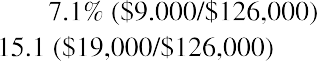• In January, the company had sales of $9,000, which wasof the total annual sales.
• In June, the company had $19,000 sales, which wasof the total annual sales and of January sales.

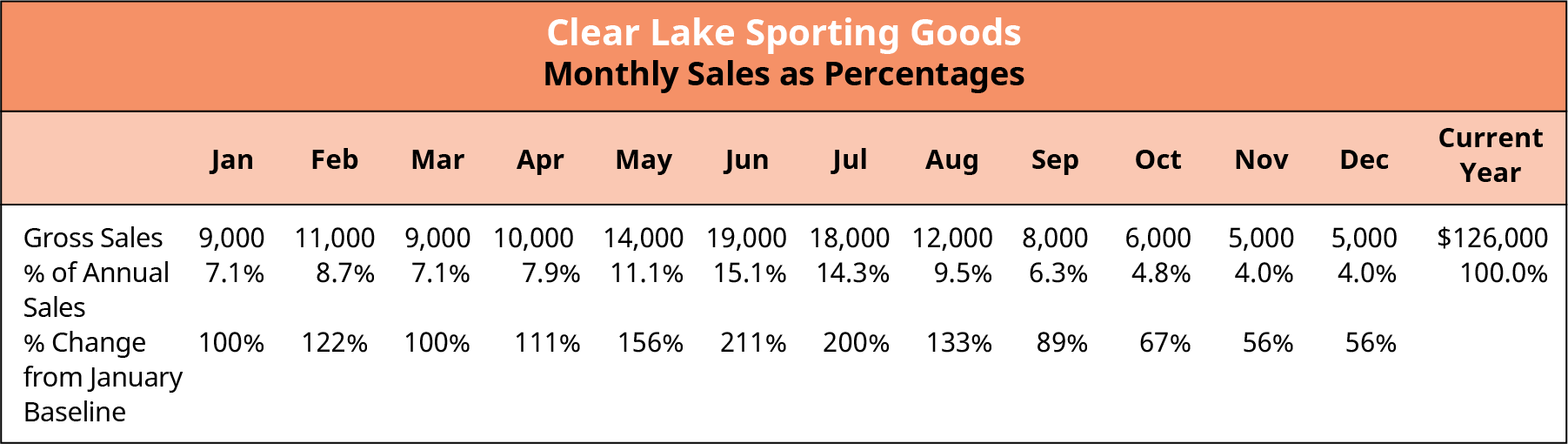
Figure 18.8 Historical Sales Data as Percentages

Once a baseline in the 12-month period is assessed, it can also be helpful to look for trends in other ways. For example, the past several years might be assessed to see if there is a trend in total growth or decline for those years on a summary basis or by period. Clear Lake Sporting Goods had sales in the current year of $126,000, in the prior year of $105,000, and two years ago of $89,000. This reflects a 20% increase and an 18% increase, respectively. It might be reasonable to expect a roughly 18 to 20% increase in total sales in the future with only this information in mind. Keep in mind that we will learn about many other factors to consider in the forecast, so the 18 to 20% increase is a good general guideline to consider along with other factors.

THINK IT THROUGHSales Forecast for Big 5 Sporting GoodsReview the 2020 annual report for Big 5 Sporting Goods (https://openstax.org/r/ 2020_annual_report_for_Big_5_Sporting_Goods). Locate the consolidated statements of operations on page F-7. Using the company’s net sales figures for the current and prior years, what percentage might you recommend for their sales forecast for the next year?Solution:Big 5’s sales for 2020 and 2019 were $1,041,212,000 and $996,495,000, respectively. This represents a 4.5% growth from the prior year. Forecasted sales, based solely on this information, might be appropriate at 4.5% growth for the next year, keeping in mind that many other factors should also be considered along with this information. Historical sales are only one set of data to use as a starting point.

Looking at Figure 18.9, assume that Clear Lake Sporting Goods decides to take its first pass at a forecast using the more conservative estimate of 18% total sales growth. The company could consider last year’s sales of

$126,000 and increase them by 18% to arrive at total forecasted sales for next year of

. Next, to get the monthly sales, the company could use the same percent of the total for each month that it did for the previous year. For example, sales in January of last year were 7.1% of the full year’s sales. To find the forecast for the next year, the company would take the forecasted sales of

$148,680 for the year and multiply that by 7.1% to get $10,620 for January. The process is repeated for each

month to get the full year.

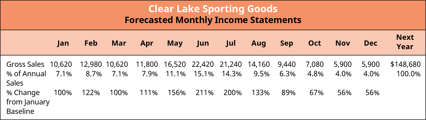
Figure 18.9 Forecasted Sales Data

Keep in mind that this is only a starting point. These estimates will be reviewed, assessed, and updated as more information and other factors are taken into consideration.

It can also be helpful to look at a shorter period, perhaps just the last few months, on a more detailed basis (by department, by customer, etc.) to see if there are any possible new trends beginning to develop that might be an indicator of performance in the coming year. For example, Clear Lake Sporting Goods might look at detailed sales records for October, November, and December and see that it had an old product line that was discontinued in early October, which contributed to a 2% reduction in monthly sales. This reduction in monthly sales will likely continue into the new year until the new line the company has signed on begins arriving in stores. Thus, the management team feels they should reduce their first quarter monthly estimates by 2%, as reflected in Figure 18.10. January is now , for example.

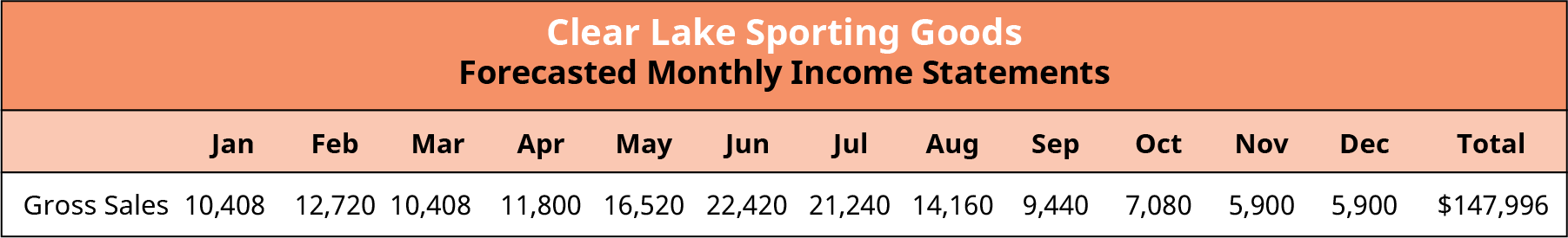
Changes for the Future

Figure 18.10 Adjusted Forecasted Sales Data

It’s important to note that the past is not always a reliable predictor of the future. Circumstances can often change to make the future quite different from the past. The business itself may change, the economy can change, the customer base may undergo a shift in demographics or a change in buying habits, new competition may emerge, and so on. So while past performance is helpful, it is only one step in the process of forecasting sales.

LINK TO LEARNINGBig 5 Sporting Goods MD&A ReportReview the most recent annual report for Big 5 Sporting Goods (https://openstax.org/r/ annual_report_for_Big_5_Sporting_Goods). Review the management’s discussion and analysis (MD&A) report (Item 7). What information does the report share about the firm, the economy, and other factors that might be useful for forecasting sales growth for next year?

Most firms first look to the past to target some form of baseline estimate for the coming year; then, managers begin making adjustments based on what they know about the future. Assume that Clear Lake Sporting Goods will be adding a new brand to its collection of fishing supplies in March. The manufacturer plans to begin running its commercials in late February, which managers anticipate will increase Clear Lake’s monthly sales

by about $500 in March, $1,000 in April, $1,400 in May, and $2,000 per month in June, July, and August. We see the monthly adjustments to Clear Lake’s latest sales forecast in Figure 18.11. March, for example, is now

$10,908 ($10,408 prior estimate plus $500 increase from new brand).

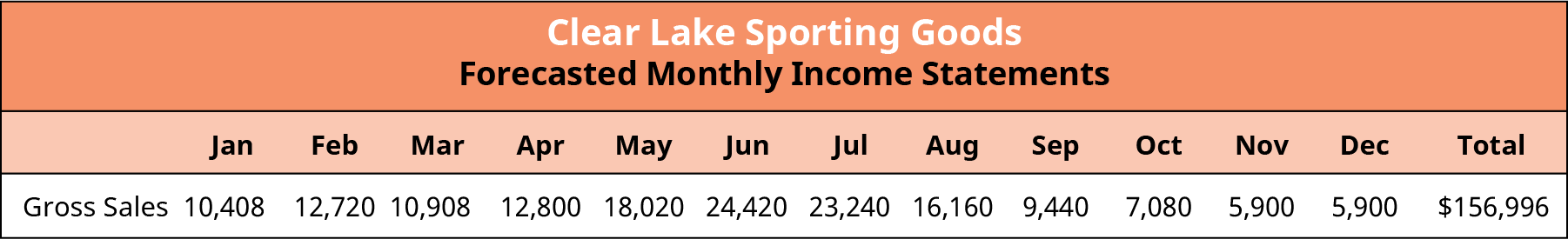
Figure 18.11 Forecasted Sales Data with New Brand

What we have discussed here are only some brief examples of the myriad factors that might impact a sales budget for the coming year. It’s critical that all members of the team take the time and effort to research their customers and the factors that impact their business in order to effectively assess the impact of these factors on future sales. Though only two adjustments were made here, it’s likely that a large firm would have to consider many, many factors that would ultimately impact monthly sales figures before arriving at a conclusion.

18.3
Pro Forma Financials

Learning Outcomes

By the end of this section, you will be able to:

• Define pro forma in the context of a financial forecast.
• Describe the factors that impact the length of a financial forecast.
• Explain the risks associated with a financial forecast.

In this section of the chapter, we will move beyond the sales forecast and look at the general nature, length, and timeline of forecasts and the risks associated with using them. We’ll look at why we use them, how long they generally are, what the key variables in a forecast are, and how we pair those variables with common-size analysis to develop the forecast.

Purpose of a Forecast

As mentioned earlier in the chapter, forecasts serve different purposes depending on who is using them. Our focus here, however, is the world of finance. In this realm, the key purpose of pro forma (future-looking) financial statements is to manage a firm’s cash flow and assess the overall value that the firm is generating through future sales growth. Growing just for the sake of growing doesn’t always yield favorable income for the firm. A larger top-line sales figure that results in lower net income doesn’t make sense in the grand scheme of things. The same is true of profitable sales that don’t generate enough cash flows at the right time. The firm may make a profit, but if it doesn’t manage the timing of its cash flows, it could be forced to shut down if it can’t cover the costs of payroll or keep the lights on. Forecasting helps assess both cash flow and the profitability of future growth. Managers can forecast cash flow using data from forecasted financial statements; this allows them to identify potential gaps in cash and plan ahead in order to either alter collection and payment policies or obtain funding to cover the gap in the timing of cash flows.

LINK TO LEARNINGPro Forma Financial StatementsReview the video Business Plan and Pro-Forma Financial Statements (https://openstax.org/r/ Business_Plan_and_Pro-Forma_Financial_Statements) to learn about the basics of pro forma financial statements and why they are helpful.

Length of a Forecast

Forecasts can generally be for any length of time. The length generally depends on the user’s needs. A one- year forecast, broken down by month, is quite typical. A firm will often go through a formal budgeting process near the end of its calendar or fiscal year to project financial plans and goals for the coming year. Once that is done, a rolling financial forecast is then done monthly to adjust as time moves on, more information becomes available, and circumstances change.

To be useful, the future forecast for financial planning purposes is almost always calculated as monthly increments rather than one total figure for the next 12 months. Breaking the data down by month allows finance managers to more clearly see fluctuations in cash flows in and out, identify potential gaps in cash flow, and plan ahead for their cash needs.

Forecasts can also be done for several years into the future. In fact, they commonly are. However, once the firm is looking out beyond 12 months, it gets difficult to forecast items with a great degree of accuracy. Often, forecasts beyond a year will be completed only to quarterly or even annual figures rather than monthly.

Forecasts that far into the future are often strategic in nature, made more to communicate future plans for the firm than for more detailed decision-making and cash flow planning.

Common-Size Financials

As we saw earlier in the chapter, common-size analysis involves using historical financial statements as a basis for future forecasts. Financial statements provide a great starting point for analysis, as we can see the relationships between sales and costs on the income statement and the relationships between total assets and line items on the balance sheet.

For example, in Figure 18.6, we saw that for the past two years, cost of goods sold has been 50% of sales. Thus, in the first draft of a forecast for Clear Lake, it’s likely that managers would estimate cost of goods sold at 50% of their forecasted sales. We can begin to see why forecasting sales first is crucial and why doing so as accurately as possible is also important.

Select Variables to Use

A simple way to begin a full financial statement forecast might be to simply use the common-size statements and forecast every item using historical percentages. It’s a logical way to begin a very rough draft of the forecast. However, several variables should be taken into consideration. First, managers must address the cost of an account and determine if it’s a variable or fixed item. Variable costs tend to vary directly and proportionally with production or sales volume. Common examples include direct labor and direct materials. Fixed costs, on the other hand, do not change when production or sales volume increases or decreases within the relevant range. Granted, if production were to increase or decrease by a large amount, fixed costs would indeed change. However, in normal month-to-month changes, fixed costs often remain the same. Common examples of fixed costs include rent and managerial salaries.

So, if we were to approach our common-size income statement, for example, we would likely use the percentage of sales as a starting point to forecast variable items such as cost of goods sold. However, fixed costs may not be accurately forecast as a percentage of sales because they won’t actually change with sales. Thus, we would likely look at the history of the dollar values of fixed costs in order to forecast them.

CONCEPTS IN PRACTICECOVID-19 Makes Forecasting Difficult for Big 5 Sporting GoodsBig 5 Sporting Goods announced record earnings in the third quarter of 2020, attributing its huge success that quarter to the impact of people’s reactions to the COVID-19 pandemic. With so many people in

quarantine still wanting to make healthy lifestyle choices, sporting goods stores were making record sales. Record-breaking sales, however, are not certain in the future. The impacts of the pandemic are extremely difficult to predict, making it a challenge for Big 5 Sporting Goods and other companies to assemble pro forma financial statements.(sources: https://www.globenewswire.com/news-release/2020/10/27/2115470/0/en/Big-5-Sporting-Goods- Corporation-Announces-Record-Fiscal-2020-Third-Quarter-Results.html; https://finance.yahoo.com/news/ investors-want-big-5-sporting-054658521.html; https://www.cpapracticeadvisor.com/accounting-audit/ news/21206691/four-ways-covid19-will-impact-2021-financial-forecasting-and-planning)

Determine Potential Changes in Variables

So far, we have focused on using historical common-size statements to create a draft (not a final version) of the forecast. This is because the past isn’t always a perfect indicator of the future, and our finances don’t always follow a linear pattern. We use the past as a good starting point; then, we must assess what else we know to fine-tune and make adjustments to the forecast.

Many items impact the forecast, and they will vary from one organization to another. The key is to do research, gather data, and look around at the market, the economy, the competition, and any other factors that have the potential to impact the future sales, costs, and financial health of the company. Though certainly not an exhaustive list, here are a few examples of items that may impact Clear Lake Sporting Goods.

• It has an old product line that was discontinued in early October, contributing to a 2% reduction in monthly sales that will likely continue into the new year until a new line begins arriving in stores.
• It will be adding a new brand to its collection of fishing supplies in March. The manufacturer plans to begin running commercials in late February. Managers anticipate that this will increase Clear Lake’s monthly sales by about $500 in March, $1,000 in April, $1,400 in May, and $2,000 per month in June, July, and August.
• The company has just finished updating its employee compensation package. It goes into effect in January of the new year and will result in an overall 4% increase in the cost of labor.
• The landlord indicated that rent will increase by $50 per month starting July 1.
• Some fixed assets will be fully depreciated by the end of March. Thus, depreciation expense will go down by $25 per month beginning in April.
• There are rumors of new regulations that will impact the costs of importing some of the more difficult-to- obtain hunting supplies. Managers aren’t entirely sure of the full impact of the new legislation at this time, but they anticipate that it could increase cost of goods sold for the affected product line when the new legislation goes into effect in the last quarter. Their best estimate is that it could increase the overall cost of goods sold by up to 2%.

We will use all of this data later in the chapter when we are ready to compile a complete forecast for Clear Lake.

18.4
Generating the Complete Forecast

Learning Outcomes

By the end of this section, you will be able to:

• Generate a forecasted income statement that incorporates pertinent sales, functional, and policy variables.
• Generate a forecasted balance sheet.
• Connect the balance sheet and income statement forecasts with appropriate feedback linkages.

In this section of the chapter, we will tie together what we have learned so far about forecasting sales,

common-size analysis, and using what we know about the company and its environment to create a full set of pro forma (forward-looking or forecasted) financial statements.

Forecast the Income Statement

To arrive at a fully forecasted income statement, we use historical income statements, common-size income statements, and any additional information we have about future sales and costs, such as the effects of the economy and competition. As we saw earlier in the chapter, we begin with forecasted sales because they are the basis for many of the forecasted costs.

Let’s begin with the sales forecast for Clear Lake Sporting Goods that we saw earlier in the chapter, in Figure 18.9, and use it along with the prior year income statement by month shown in Figure 18.12. We will consider other data we have about the business to begin creating a full income statement (see Figure 18.13).

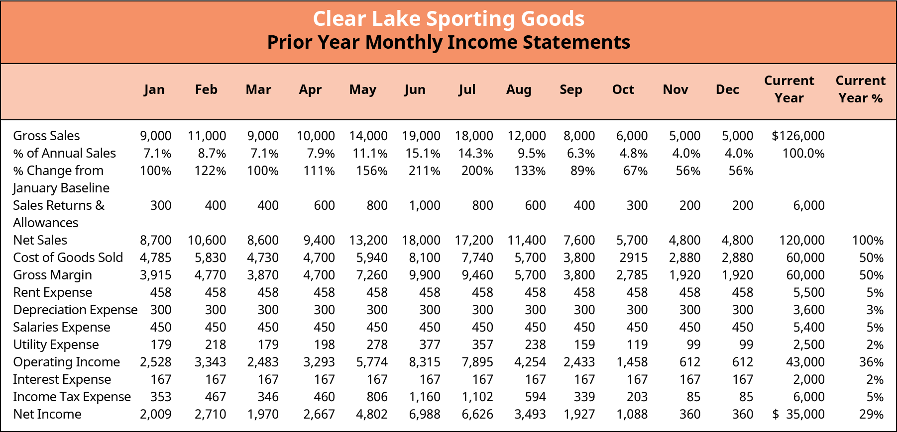
Figure 18.12 Prior Year Monthly Income Statement by Month

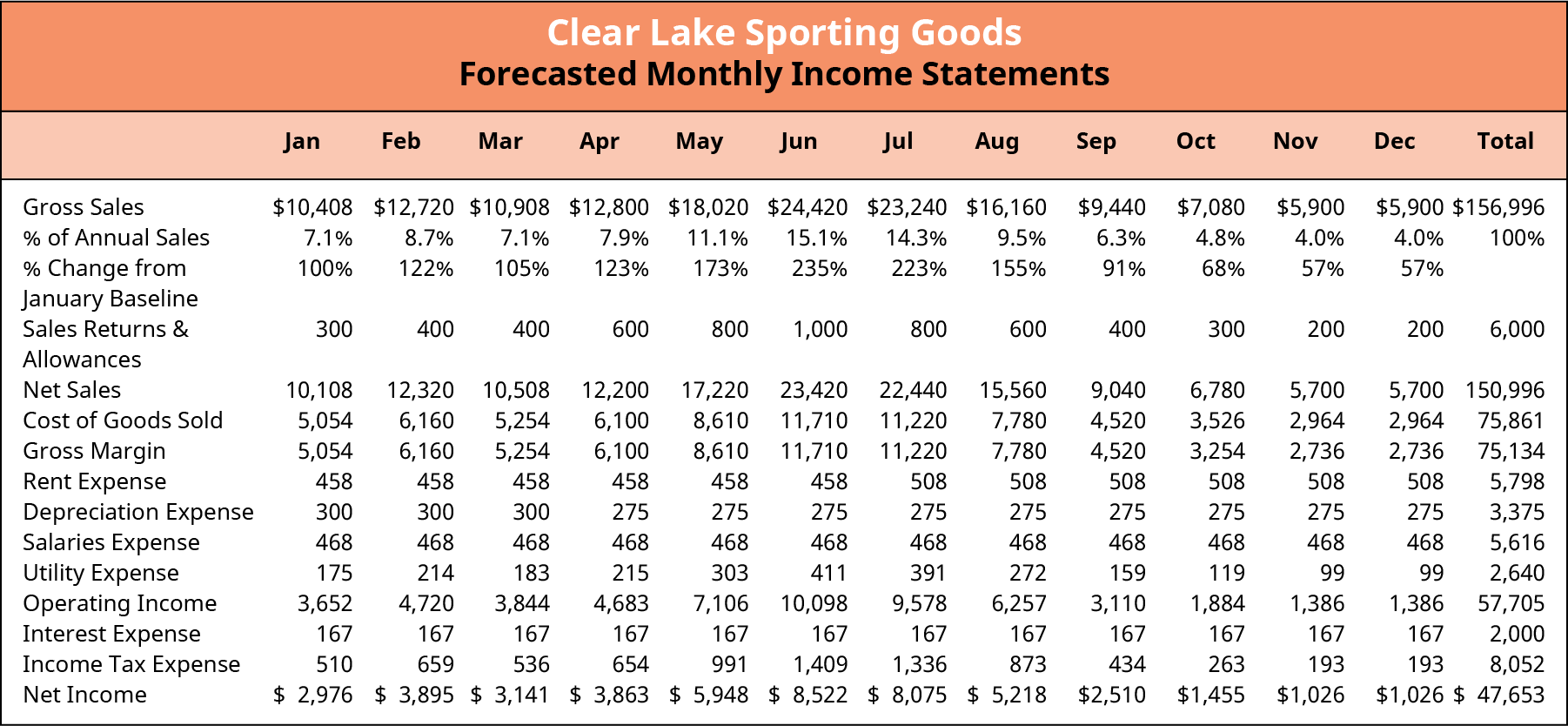
The first two key points regarding product lines have already been built into the sales forecast. Notice that the cost of goods sold was 50% in the prior year. However, based on possible future legislation, to be conservative, we should increase the cost of goods sold by 2% in the last quarter of the year. Thus, we will forecast cost of goods sold at 50% of sales in the first nine months and increase it to 52% in the last three months of the year.

Rent is a fixed cost that historically amounts to $458 per month. However, we know that the landlord is increasing rent by $50 starting on July 1. Thus, we will forecast rent at the same fixed cost of $458 per month for the first six months and increase it to $508 per month for the second half of the year.

Depreciation, also a fixed cost, was historically $300 per month. However, we know that depreciation expense will go down by $25 beginning in April. Thus, we forecast depreciation at $300 for the first three months and at

$275 for the last 9 months.

Salaries expense has historically been $450 per month. However, we know that the company is implementing a new compensation program on January 1 that will increase salaries expense by 4% ($18). Thus, we will forecast salaries for the whole year at $468.

Utilities expense seems to vary somewhat by sales from month to month, as shops are open longer hours during their busy season. However, the total utilities expense is not expected to change for the coming year. Thus, the forecast for utilities expense remains at $2,500, broken down by month as a percentage of sales.

Interest expense is a fixed cost and isn’t anticipated to change. Thus, the same $167 interest expense per month is forecast for the coming year.

Finally, income tax expense is forecasted as a percentage of operating income because tax liability is incurred as a direct result of operating income. Figure 18.13 shows the next 12 months’ forecast for Clear Lake Sporting Goods using all of this data.

Forecast the Balance Sheet

Figure 18.13 Forecasted Income Statement

Now that we have a reasonable income statement forecast, we can move on to the balance sheet. The balance sheet, however, is entirely different from the income statement. It requires a bit more research and additional assumptions. Just like the income statement, it’s often a work in progress. A first draft is a good starting point, but adjustments must be made once it is created, and all the interrelationships between the statements, cash flow in particular, are taken into consideration.

The balance sheet is a bit more difficult to forecast because the statement reflects balances at just a given point in time. Account balances change daily, so forecasting just one snapshot in time for each month can be a challenge. A good starting point is to assess general company financial policies or rules of thumb. For example, assume that Clear Lake pays most of its vendors on net 30-day terms. A good way to forecast accounts payable on the balance sheet might be to add up the cost of goods sold from the forecasted income statement for the prior month. For example, in Figure 18.14, we see that Clear Lake has forecasted its accounts payable for March as the cost of goods sold in March from its forecasted income statement.

For accounts receivable, Clear Lake generally receives payment from customers within net 90-day terms. Thus, it uses the sum of the current and prior two months’ forecasted sales to estimate its accounts receivable balance.

Inventory will vary throughout the year. For the first six months, the company tries to build inventory for four months of sales. Once the busy season hits, inventory goes down to three months’ worth of future sales, then finally drops to only two months of sales in December. Thus, managers use their sales forecast by month to estimate their inventory ending balance each month.

The equipment balance is forecasted by reducing the prior month’s balance by the forecasted depreciation expense on the forecasted income statement.

Unearned revenue is historically around 50% of the current month’s sales. Thus, Clear Lake estimates its unearned revenue balance each month by taking the current month’s net sales from the forecasted income statement and multiplying it by 50%.

Short-term investments, notes payable, and common stock are not anticipated to change, so the current balance is forecasted to remain the same for the next 12 months.

To forecast the ending balance for retained earnings for each month, managers add the monthly net income from the forecasted balance sheet to the prior balance and subtract a quarterly $10,000 dividend.

Once all of these accounts are completed, the balance sheet is out of balance. Given that all of these events are somewhat related but are not tied together dollar for dollar, it’s not surprising when the forecasted balance sheet is finished and does not balance. To complete the first draft (see Figure 18.14), the cash account is used as a variable and plugged in to make the balance sheet balance. Notice that by the end of the year, the company has $59,905 in cash. However, look at what happens midyear—the cash account falls to only $8,782. In the next section, we will generate a cash flow forecast, which will allow Clear Lake to update its balance sheet forecast once it estimates what it will do to cover the cash flow gaps.

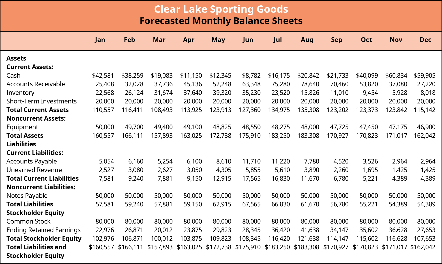
Figure 18.14 Forecasted Balance Sheet Draft

Linkages between the Forecasted Balance Sheet and the Income Statement

Notice that in the discussion in the prior section on the balance sheet forecast, a lot of the information in the forecasted income statement was used to generate the forecasted balance sheet. The balance sheet accounts generally depend on activity reported in the income statement. For example, for many firms, the balance in their accounts receivable account is tied to their sales. Looking at historical balances in the accounts receivable account and how those relate to historical sales will help determine how to use the forecasted future sales to estimate the future balance of accounts receivable.

The same is true of accounts payable. Looking at past balances, past expenses (normally cost of goods sold), and the firm’s payment terms for its vendors allows managers to use forecasted cost of goods sold or other expenses to estimate the balance in the accounts payable account.

We learned in Financial Statements that net income flows into retained earnings. Thus, the net income from the forecasted income statement can be used to help estimate the ending balance in retained earnings. If the firm intends to issue any dividends in the coming year, managers should also estimate that reduction in their forecast.

It’s also common to find other general policies or procedures that help drive performance and aid in forecasting balances. For example, if the company has a goal of maintaining a certain level of inventory or a minimum balance in its cash account, that information can be used to guide the estimate for those accounts.

18.5
Forecasting Cash Flow and Assessing the Value of Growth

Learning Outcomes

By the end of this section, you will be able to:

• Generate a cash flow forecast.
• Assess a cash flow forecast to determine future cash funding needs.
• Use pro forma financial statements and cash flow forecasts to assess the value of growth to the firm.

In this section of the chapter, we will use the forecasted income statement, forecasted balance sheet, and other information we know about the firm’s policies and goals for the coming year to generate and assess a cash flow forecast.

Create a Cash Flow Forecast

A cash flow forecast isn’t overly complex, yet it is not easy to assemble because it requires making many assumptions about the future. A cash forecast begins with the beginning cash balance, adds anticipated cash inflows, and deducts anticipated cash outflows. This identifies cash surpluses and shortages.

For Clear Lake Sporting Goods, for example, we see in Figure 18.15 that the company begins with cash of

$42,581,000 in January of the new year. Next, it lists the cash inflows, or cash received from customers. Given the assumption that customers pay in 90-day terms, the cash flow is filled in by plugging in the sales forecast for the three prior months. For example, the cash flow from customers of $10,508 for June is the same as the net sales forecast for March (see Figure 18.13).

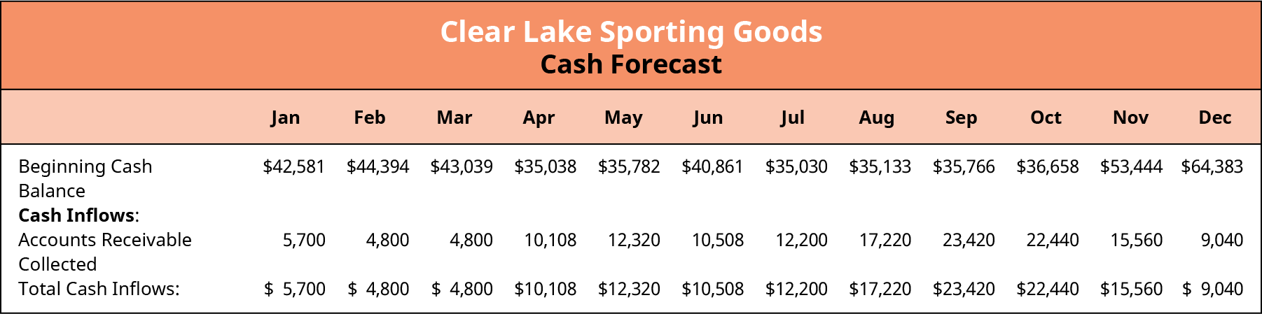
Figure 18.15 Forecasted Cash Inflows

Next, Clear Lake identifies cash outflows, which include accounts payable, salaries, rent, utilities, dividends, and interest payments. Accounts payable are normally paid within 30 days, so the forecast for cost of goods sold for the prior month is used as an estimate of amount paid for payables. For example, in Figure 18.16, we see that the accounts payable settled in June of $8,610 is the cost of goods sold for May from the forecasted income statement.

Salaries are paid monthly and thus represent the same recurring monthly cash outflow, as does rent. Utilities, like accounts payable, are assumed to be paid within 30 days. Thus, the cash outflow for utilities is the utilities expense for the prior month from the forecasted income statement.

Management intends to pay a quarterly dividend of $10,000. Thus, in Figure 18.16, we see $10,000 cash outflows forecasted for March, June, September, and December. Interest on the long-term liability is paid quarterly. Thus, the $500 cash outflows in March, June, September, and December are simply the monthly interest expense of $167 from the income statement, summed for each quarter.

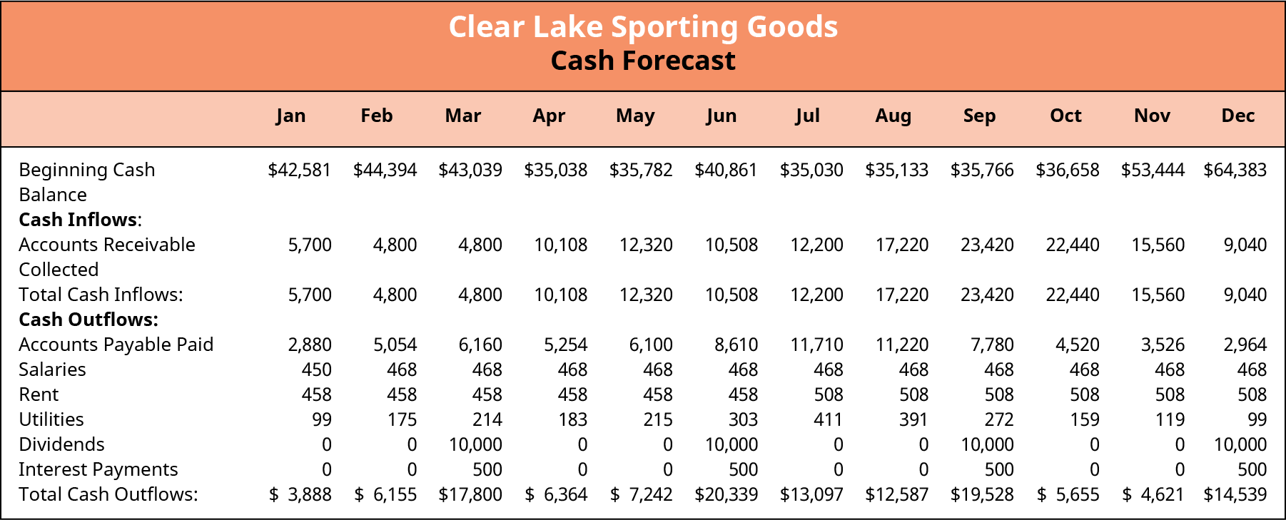
Figure 18.16 Forecasted Cash Inflows and Outflows

Using a Cash Forecast to Determine Additional Funds Needed

Finally, at the end of the cash flow forecast, cash outflows are subtracted from the cash inflows. This identifies whether a cash surplus (extra) or cash deficit (not enough) exists for each month. For example, in Figure 18.17, we see that in March, Clear Lake is forecasting $4,800 of cash inflows and $17,800 of total cash outflows, which results in a cash deficit of $13,000.

Clear Lake has a general policy to not let its cash balance fall below $35,000. Thus, managers need to assess their monthly balances and potential deficits and identify months when financing is necessary. For example, the deficit of $13,000 in March is enough to push the cash balance lower than $35,000. Thus, it’s estimated that the company will need $5,000 in short-term financing in March. It has an estimated surplus in April, so $3,000 of the borrowing is returned.

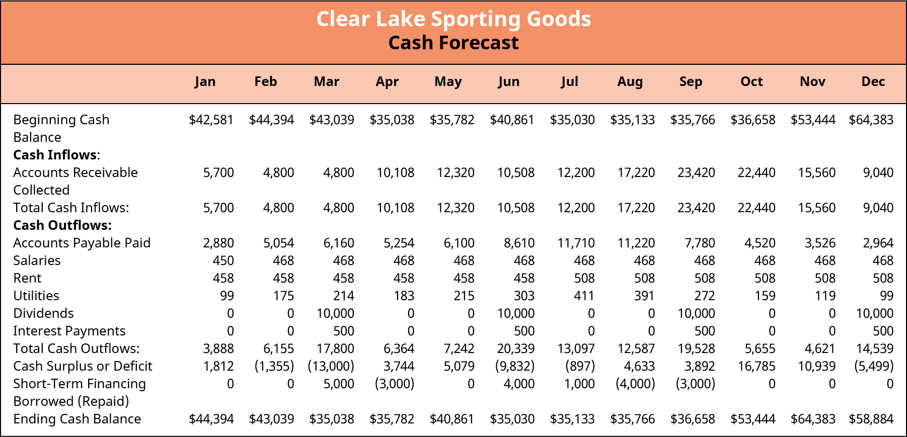
Figure 18.17 Forecasted Cash Surplus or Deficit

Assessing the Value of Growth

It’s a fairly common assumption that most, if not all, businesses want to grow. While it certainly can be good as a firm to grow in size, growth just for the sake of growth isn’t necessarily a good goal. A firm can grow in size based on customers, employees, locations, or simply sales. However, that doesn’t mean that the growth will increase profits. Growth may increase profits, but this is not a safe assumption. Scaling up operations takes careful planning, which includes monitoring the profitability of the sales and, of course, the cash flow it

would require. Growing a business can require more inventory, more locations, more equipment, and more manpower, all of which cost money. Even if the forecasted growth is profitable, it may pose problems from a cash flow perspective. It’s important that the firm review not only its forecasted income statement and balance sheet but also its cash forecast, as this can reveal some serious gaps in funding depending on the extent, timing, and nature of the planned growth.

For example, assume that Clear Lake Sporting Goods intends to run a large-scale ad campaign to boost sales in its busy season. Historically, the store relied primarily on its prime location for high volumes of retail foot traffic. Managers felt, however, that given the increase in competition, they could boost sales significantly by running the ad campaign in the first quarter. The campaign would cost $30,000. Forecasts already reflect a cash deficit at the end of the first quarter of $13,000, so the additional $30,000 ad campaign, which would require payment up front, would create a much larger need for funding. It’s also important that managers look at the increased cost of doing business along with the increased cost in advertising to ensure that the move would be profitable. Fortunately, Excel or other forecasting software can be used to create a forecast with formulas that tie together, making scenario analysis such as this a much easier process.

Scenarios in Forecasting

Forecasting is almost never a linear process. In other words, we don’t do one forecast and call it good. The first draft is completed using historical data, and then changes are made a bit at a time as all potential variables are assessed for their impact on the forecast. It’s quite common to then use the work-in-progress forecast to complete scenario analysis. This is particularly true when the forecast is completed in Excel or other budgeting or forecasting software. Elements of the forecast can be changed to see what the overall impact would be to the firm. Assuming the forecast is set up using formulas in Excel or other software, a change to one figure or one variable would then “ripple” through the forecast to reflect the overall impact.

Often, a firm may complete an initial forecast (scenario) under the assumption that the economy is in a “normal state.” The firm can then alter the initial forecast for different scenarios, such as the economy in a recession or the economy in a state of expansion. This helps the firm understand different possible future states and highlights how changes in the economy such as inflation may cause revenue and expenses to increase.

Assume that Clear Lake’s initial forecast is created under the assumption that the economy will remain average. Management also wants to know the worst-case scenario. What will their financial results look like if the economy were in a recession, for example? If management assumes their sales would drop to only 60% of the prior year sales in a recessionary economy, they could alter the formula in Excel driving their sales and variable costs, resulting in a new pro forma income statement. In Figure 18.18, we can see that net income would drop to $16,391 under this assumption, compared to the net income of $47,653 forecasted under average economy assumptions in Figure 18.13.

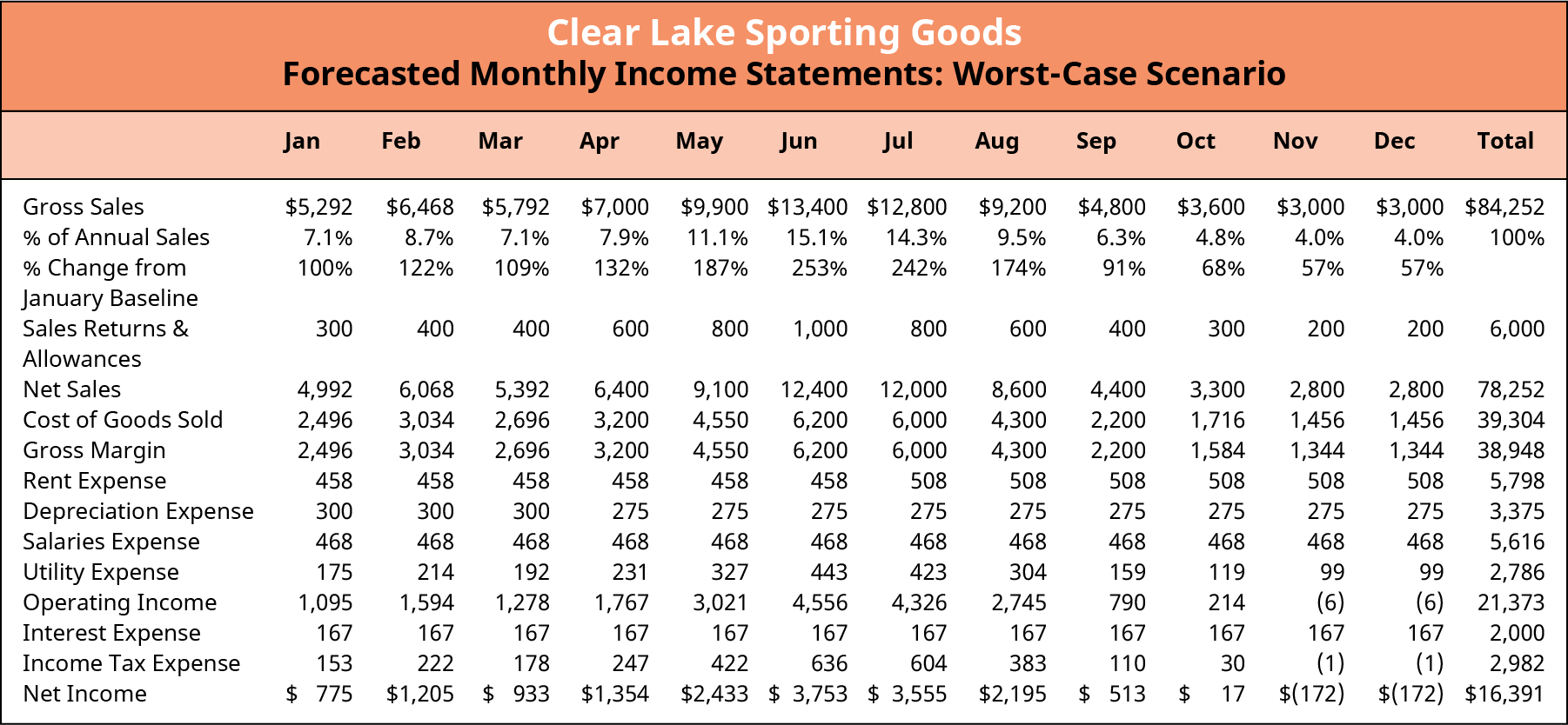
Figure 18.18 Forecasted Cash Surplus or Deficit

Though creating a full forecast in Excel can be a bit complex, it is a powerful tool that is useful for analysis. Elements can be used to vary just about anything, from something small such as a 1% increase in the cost of a product to a company-wide increase in salaries, the introduction of an entire new product line, or the purchase of a new production machine, among other possibilities.

For example, assume that Clear Lake has completed a first pass at its forecast and is reviewing the forecasted profit for the next 12 months. Managers feel the profit is currently low, as they always want to target a certain percentage. They might tinker with variables in the forecast file to see the impact on profits of potential changes they are considering. They may reduce the new salaries package by a percentage point to see if it gets them closer to their goal. They may adjust cost of goods sold by a certain percentage if they feel they can negotiate with vendors to work down their costs. They may adjust rent and see if they can find a better retail location to either reduce costs or increase sales due to increased foot traffic in a new location. They may save an entirely new version of the forecast and change it drastically to see what investing in opening a second retail location would do.

As you can see, the list of possibilities is endless. Though the main goal of financial managers may be cash planning, the power of a well-developed forecast is tremendous. It can help assess potential growth, new opportunities, and even small changes in the business as well.

Sensitivity Analysis in Forecasting

Sensitivity analysis will often look at the change in just one variable rather than the entire scenario. It examines how sensitive a particular output (commonly net income) will be to a change in a particular underlying input (sales or costs, for example). What if sales are 10% more or less than forecasted? What if the prices the firm can charge its customers are 10% more or less? What if the cost of goods sold increases by 10%? The purpose is to see which variables are crucial to “get right.” It isn’t worth spending a lot of research dollars to make sure you are accurately predicting a variable if that variable won’t notably change the outcome. However, a slight change in other variables may have significant impact.

Using pro forma financial statements created in Excel allows management to quickly generate new pro forma financials and see the impact that each possible variable might have on the overall financial results.

18.6
Using Excel to Create the Long-Term Forecast

Learning Outcomes

By the end of this section, you will be able to:

• Generate a financial statement forecast using spreadsheet tools.
• Connect the balance sheet and income statement using appropriate formula referencing.
• Use spreadsheet functions to generate appropriate iterations that balance financial forecasts.

Throughout this chapter, we have seen forecasted financial statements for Clear Lake Sporting Goods along with its forecasted cash flow. These statements could all have been generated by hand, of course, but that wouldn’t be an effective use of time. As mentioned in prior sections, several different types of software can be quite effective in making the forecasting process faster and more flexible. In this section, we will review just one common option, Microsoft Excel.

Download the spreadsheet file (https://openstax.org/r/spreadsheet_file) containing key Chapter 18 Excel exhibits.

Using the “Sheet”

Creating a budget in Excel can be very simple or extremely complex, depending on the size and complexity of the business and the number of formulas and dependencies that are written into the Excel workbook.

Creating the forecast in Excel follows the same steps and flow we just explored in this chapter but with the power of a software program to do the math for you. We begin with the sales forecast, which uses several key formulas in Excel.

• First, sales are projected to be 18% higher than the prior year. Thus, a total projection for the year is calculated using a simple link and multiplication function tied to last year’s total sales. In Figure 18.19, you can see the formula in cell O4 is “=’Figure 18.12′!N4*1.18”. This formula simply does the math to increase the prior year’s sales by 18%.
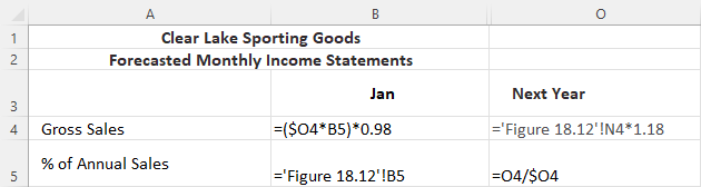• Next, the sales are distributed by month. In Figure 18.19, we see in cell B5 that the forecasted income statement sheet is linked to the percent of annual sales from the Prior Year Income Statement (Figure 18.12) sheet. Then, in cell B4, January sales are estimated with a formula that multiplies the total forecasted sales in O4 by the percent of annual sales for January of the prior year. Notice that the formula then multiplies that product by 0.98. This is because Clear Lake discontinued a product line in the last quarter of the prior year, and management feels that this will reduce sales in the first quarter of the new year by roughly 2%.

Figure 18.19 Forecasted Sales Formulas in Excel

• As Clear Lake continues to fill out its forecasted income statement, the next formula we see is a simple sum formula to calculate net sales in B8 (see Figure 18.20). It’s a simple formula that subtracts sales returns and allowances in B7 from gross sales in B4. Similar formulas are also found in B10 for gross margin and B18 for net income.
• In cell B9, we see a multiplication formula that multiplies sales from B4 by 0.5, or 50%. This is because

management feels that cost of goods sold will remain the same as last year, in most quarters at least, and last year’s percentage was 50%.

• Rent, depreciation, and salaries are all simply typed in, as they are fixed expenses that remain the same as last year.
• The utilities calculation, found in cell B14, is somewhat similar to the sales calculation. The total utilities expense from O14 is multiplied by the current month’s sales in B4 divided by the total annual sales in O4. This spreads out the utility cost by month based on the percentage of annual sales.

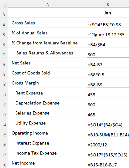
Figure 18.20 Forecasted Income Statement Formulas

Clear Lake’s forecasted balance sheet ties very closely to both the forecasted income statement and the prior year’s income statement. In Figure 18.21, we see in C7 an addition formula using the sum of the current month and three months of prior sales as an estimate of the ending accounts receivable balance. The formula for inventory is similar but forward looking. In C8, inventory is estimated by adding the cost of goods sold for the current month and next three months from the forecasted income statement.

Total current assets in C10 is calculated with a SUM formula that adds together the values in all the selected cells. Amounts such as short-term investments and common stock that are not anticipated to change are simply typed as a number in the cell. Much like in the income statement, subtotals are found in C13 for total assets, C17 for current liabilities, C24 for total equity, and C25 for total liabilities and equity. Retained earnings in C23 pulls the ending retained earnings balance from the end of last year (hidden in column B) and adds the

net income for January in the forecasted income statement to get the current month’s ending balance.

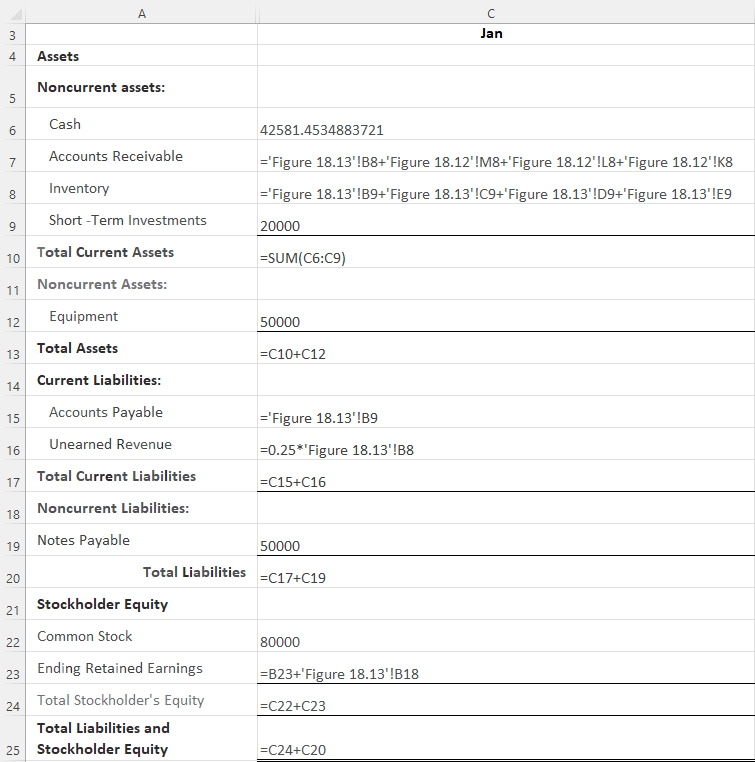
Figure 18.21 Forecasted Balance Sheet Formulas

Much like the balance sheet, the cash forecast also relies heavily on data from the forecasted income statement as well as the forecasted balance sheet. To begin the year, in Figure 18.22, we see that the formula in B4 pulls the cash balance from the forecasted balance sheet. In B6, the formula pulls the sales for the three months prior from the previous year’s income statement. This is because it’s assumed that cash is collected from customers 90 days after the sale. The same approach is used for accounts payable, rent, salaries, and utilities. The formulas pull the expenses from a prior month depending on the assumed timing for payment. Utilities, for example, are assumed to be paid within 30 days, so the cash outflow in February is assumed to be the utilities expense for January from the forecasted income statement. Note that interest payments are assumed to be zero in January and February, but in March, the formula in D14 sums the interest expenses on the forecasted income statement for January, February, and March. This is because interest is paid quarterly.

Finally, note the formula in C4. The beginning cash balance for a given month is the same as the ending cash balance from the prior month; thus, the figure in B18 is linked to C4 to start the new month.

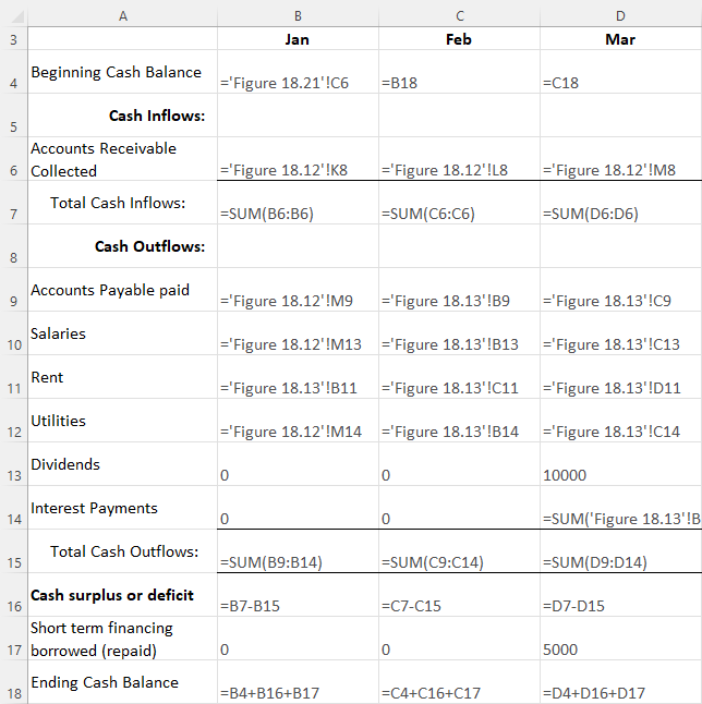
Figure 18.22 Cash Forecast Formulas

Using Excel Functions to Balance

Once we get a draft of the forecasts outlined, then the tinkering starts. Additional information can be used to adjust the formulas, as we saw with the 2% reduction in January sales for the forecasted income statement. Because we have linked most (though not all) of our expenses, subtotals, and statements together using formulas, management can also use the forecast workbook to perform scenario and sensitivity analyses, essentially asking “what if?” and looking at the results. When completed, however, before finalizing the forecast, it’s important that the financial statements are in balance (particularly the balance sheet, just as the name implies).

Notice that throughout, we used formulas to calculate subtotals to ensure they are correct and change as needed. We also linked figures, such as the ending and beginning cash balances, to ensure they are in balance. Perhaps the easiest but most important thing to do is to ensure that the balance sheet balances. We can do this with a simple formula that compares total assets to total liabilities and equity. We can see in Figure 18.23 that subtracting one from the other in cell C27 should result in $0. If there is a difference, the formula will highlight it, forcing us to investigate and correct the sheet so that it balances.

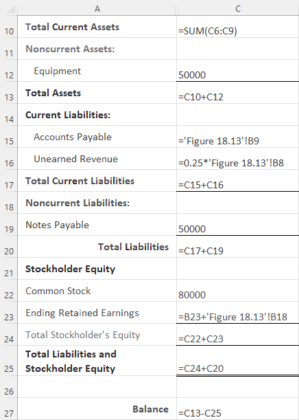
Figure 18.23 Forecasted Balancing Formula

Summary

The Importance of Forecasting

Forecasting financial statements is important to different users for different reasons. In finance, it’s most important for assessing the value of future growth plans and planning for future cash flow needs.

Forecasting Sales

The sales forecast is the foundation on which much of the rest of the forecast is built. Thus, the sales forecast is completed first. Historical sales data and any other information on the firm, its products, the economy, its customers, and its competitors are all used to create the most accurate sales forecast possible.

Pro Forma Financials

Pro forma financial statements are forward looking in nature. They use the sales forecast, historical data, financial statement analyses, relationships between accounts and statements, and any other information known about the firm, the environment, and the future to create the most accurate financial statement forecast possible.

Generating the Complete Forecast

Interrelationships among historical data, the forecasted income statement, and the forecasted balance sheet are all used to estimate each line item in the financial statements.

Forecasting Cash Flow and Assessing the Value of Growth

Once the income statement and balance sheet forecasts are complete, data from those statements, information on company policies, and account relationships are used to generate a cash forecast. The cash forecast is important for identifying any gaps in cash flow so that financial managers can plan for cash needs. It’s also important to review not only the cash forecast but all forecasted financial statements to assess the overall impact and value of proposed firm growth.

Using Excel to Create the Long-Term Forecast

Excel can be a powerful tool for creating financial forecasts. Formulas that complete mathematical functions and tie accounts and financial statements together are used to create the statements, ensure that they balance, and facilitate scenario and sensitivity analyses.

Key Terms

balance sheet a financial statement that reflects a firm’s asset, liability, and equity account balances at a given point in time

cash deficit an excess of cash outflows over cash inflows for a given period

cash forecast a financial statement that estimates a firm’s future cash inflows and outflows

cash surplus an excess of cash inflows over cash outflows for a given period

common-size describes a financial statement in which each element is expressed as a percentage of a base amount

financing activities cash business transactions reported on the statement of cash flows that reflect the use of financed funds

forecast an estimate of future performance based on historical performance and other contextual information

income statement a financial statement that measures a firm’s financial performance over a given period of time

investing activities cash business transactions reported on the statement of cash flows that reflect the acquisition or disposal of long-term assets

operating activities cash business transactions reported on the statement of cash flows that relate to ongoing day-to-day operations

pro forma in the context of financial statements, forward-looking

scenario analysis analysis of how various situations and circumstances would impact the financial forecast sensitivity analysis analysis of the sensitivity of an output variable to a change in an input variable statement of cash flows a financial statement that lists a firm’s cash inflows and outflows over a given

period of time

statement of stockholders’ equity a financial statement that reports the difference between the beginning and ending balances of each of the stockholders’ equity accounts during a given period