15 Lesson 10 Capital Budgeting
One of the most important decisions a company faces is choosing which investments it should make. Should an automobile manufacturer purchase a new robot for its assembly line? Should an airline purchase a new plane to add to its fleet? Should a hotel chain build a new hotel in Atlanta? Should a bakery purchase tables and chairs to provide places for customers to eat? Should a pharmaceutical company spend money on research for a new vaccine? All of these questions involve spending money today to make money in the future.
The process of making these decisions is often referred to as capital budgeting. In order to grow and remain competitive, a firm relies on developing new products, improving existing products, and entering new markets. These new ventures require investments in fixed assets. The company must decide whether the project will generate enough cash to cover the costs of these initial expenditures once the project is up and running.
For example, Sam’s Sporting Goods sells sporting equipment and uniforms to players on local recreational and school teams. Customers have been inquiring about customizing items such as baseball caps and equipment bags with logos and other designs. Sam’s is considering purchasing an embroidery machine so that it can provide these customized items in-house. The machine will cost $16,000. Purchasing the embroidery machine would be an investment in a fixed asset. If it purchases the machine, Sam’s will be able to charge customers for customization.
The managers think that selling customized items will allow the company to increase its cash flow by $2,000 next year. They predict that as customers become more aware of this service, the ability to customize products in-house will increase the company’s cash flow by $4,000 the following year. The managers expect the machine will be used for five years, with the embroidery products increasing cash flows by $5,000 during each of the last three years the machine is used. Should Sam’s Sporting Goods invest in the embroidery machine? In this chapter, we consider the main capital budgeting techniques Sam’s and other companies can use to evaluate these types of decisions.
 16.1
16.1
Payback Period Method
Learning Outcomes
By the end of this section, you will be able to:
- Define payback period.
- Calculate payback period.
- List the advantages and disadvantages of using the payback period method.
The payback period method provides a simple calculation that the managers at Sam’s Sporting Goods can use to evaluate whether to invest in the embroidery machine. The payback period calculation focuses on how long it will take for a company to make enough free cash flow from the investment to recover the initial cost of the investment.
Payback Period Calculation
In order to purchase the embroidery machine, Sam’s Sporting Goods must spend $16,000. During the first year, Sam’s expects to see a $2,000 benefit from purchasing the machine, but this means that after one year, the company will have spent $14,000 more than it has made from the project. During the second year that it uses the machine, Sam’s expects that its cash inflow will be $4,000 greater than it would have been if it had not had the machine. Thus, after two years, the company will have spent $10,000 more than it has benefited from the machine. This process is continued year after year until the accumulated increase in cash flow is $16,000, or equal to the original investment. The process is summarized in Table 16.1.
|
0 |
1 |
2 |
3 |
4 |
5 |
|
|
Initial Investment ($) |
(16,000) |
|
|
|
|
|
|
Cash Inflow ($) |
– |
2,000 |
4,000 |
5,000 |
5,000 |
5,000 |
|
Accumulated Inflow ($) |
– |
2,000 |
6,000 |
11,000 |
16,000 |
21,000 |
|
Balance ($) |
(16,000) |
(14,000) |
(10,000) |
(5,000) |
– |
5,000 |
Table 16.1
Sam’s Sporting Goods is expecting its cash inflow to increase by $16,000 over the first four years of using the embroidery machine. Thus, the payback period for the embroidery machine is four years. In other words, it takes four years to accumulate $16,000 in cash inflow from the embroidery machine and recover the cost of the machine.
LINK TO LEARNINGCalculating the Payback PeriodIt is possible that a project will not fully recover the initial cost in one year but will have more than recovered its initial cost by the following year. In these cases, the payback period will not be an integer but
will contain a fraction of a year. This video demonstrates how to calculate the payback period (https://openstax.org/r/how-to-calculate) in such a situation.
Advantages
The principal advantage of the payback period method is its simplicity. It can be calculated quickly and easily. It is easy for managers who have little finance training to understand. The payback measure provides information about how long funds will be tied up in a project. The shorter the payback period of a project, the greater the project’s liquidity.
Disadvantages
Although it is simple to calculate, the payback period method has several shortcomings. First, the payback period calculation ignores the time value of money. Suppose that in addition to the embroidery machine, Sam’s is considering several other projects. The cash flows from these projects are shown in Table 16.2. Both Project B and Project C have a payback period of five years. For both of these projects, Sam’s estimates that it will take five years for cash inflows to add up to $16,000. The payback period method does not differentiate between these two projects.
|
0 |
1 |
2 |
3 |
4 |
5 |
6 |
|
|
Project A ($) |
(16,000) |
2,000 |
4,000 |
5,000 |
5,000 |
5,000 |
5,000 |
|
Project B ($) |
(16,000) |
1,000 |
2,000 |
3,000 |
4,000 |
6,000 |
– |
|
Project C ($) |
(16,000) |
6,000 |
4,000 |
3,000 |
2,000 |
1,000 |
– |
|
Project D ($) |
(16,000) |
1,000 |
2,000 |
3,000 |
4,000 |
6,000 |
8,000 |
Table 16.2
However, we know that money has a time value, and receiving $6,000 in year 1 (as occurs in Project C) is preferable to receiving $6,000 in year 5 (as in Projects B and D). From what we learned about the time value of money, Projects B and C are not identical projects. The payback period method breaks the important finance rule of not adding or comparing cash flows that occur in different time periods.
A second disadvantage of using the payback period method is that there is not a clearly defined acceptance or rejection criterion. When the payback period method is used, a company will set a length of time in which a project must recover the initial investment for the project to be accepted. Projects with longer payback periods than the length of time the company has chosen will be rejected. If Sam’s were to set a payback period of four years, Project A would be accepted, but Projects B, C, and D have payback periods of five years and so would be rejected. Sam’s choice of a payback period of four years would be arbitrary; it is not grounded in any financial reasoning or theory. No argument exists for a company to use a payback period of three, four, five, or any other number of years as its criterion for accepting projects.
A third drawback of this method is that cash flows after the payback period are ignored. Projects B, C, and D all have payback periods of five years. However, Projects B and C end after year 5, while Project D has a large cash flow that occurs in year 6, which is excluded from the analysis. The payback method is shortsighted in that it favors projects that generate cash flows quickly while possibly rejecting projects that create much larger cash flows after the arbitrary payback time criterion.
Fourth, no risk adjustment is made for uncertain cash flows. No matter how careful the planning and analysis, a business is seldom sure what future cash flows will be. Some projects are riskier than others, with less certain cash flows, but the payback period method treats high-risk cash flows the same way as low-risk cash flows.
16.2
Net Present Value (NPV) Method
Learning Outcomes
By the end of this section, you will be able to:
- Define net present value.
- Calculate net present value.
- List the advantages and disadvantages of using the net present value method.
- Graph an NPV profile.
Net Present Value (NPV) Calculation
Sam’s purchasing of the embroidery machine involves spending money today in the hopes of making more money in the future. Because the cash inflows and outflows occur in different time periods, they cannot be directly compared to each other. Instead, they must be translated into a common time period using time value of money techniques. By converting all of the cash flows that will occur from a project into present value, or current dollars, the cash inflows from the project can be compared to the cash outflows. If the cash inflows exceed the cash outflows in present value terms, the project will add value and should be accepted. The difference between the present value of the cash inflows and the present value of cash outflows is known as net present value (NPV).
The equation for NPV can be written as


Consider Sam’s Sporting Goods’ decision of whether to purchase the embroidery machine. If we assume that after six years the embroidery machine will be obsolete and the project will end, when placed on a timeline, the project’s expected cash flow is shown in Table 16.3:
|
0 |
1 |
2 |
3 |
4 |
5 |
6 |
|
|
Cash Flow ($) |
(16,000) |
2,000 |
4,000 |
5,000 |
5,000 |
5,000 |
5,000 |
Table 16.3
Calculating NPV is simply a time value of money problem in which each cash flow is discounted back to the present value. If we assume that the cost of funds for Sam’s is 9%, then the NPV can be calculated as


Because the NPV is positive, Sam’s Sporting Goods should purchase the embroidery machine. The value of the firm will increase by $2,835.63 as a result of accepting the project.
Calculating NPV involves computing the present value of each cash flow and then summing the present values of all cash flows from the project. This project has six future cash flows, so six present values must be computed. Although this is not difficult, it is tedious.
A financial calculator is able to calculate a series of present values in the background for you, automating much of the process. You simply have to provide the calculator with each cash flow, the time period in which each cash flow occurs, and the discount rate that you want to use to discount the future cash flows to the present.
Follow the steps in Table 16.4 for calculating NPV:
Step1234Description Select cash flow worksheet Clear the cash flow worksheet Enter initial cash flowEnter cash flow for the first yearEnterCFCF02ND [CLR WORK] CF0DisplayXXXX016000 +/- ENTER CF0 = -16,000.00↓↓2000 ENTER5Enter cash flow for the second year ↓↓4000 ENTER6Enter cash flow for the third year7Enter cash flow for the fourth year8Enter cash flow for the fifth year9Enter cash flow for the sixth year↓↓↓↓↓↓↓↓5000 ENTER5000 ENTER5000 ENTER5000 ENTERSelect NPVEnter discount rateCompute NPVNPV9 ENTER↓CPTC01 =2,000.00F01 =1.0C02 =4,000.00F02 =1.0C03 =5,000.00F03 =1.0C04 =5,000.00F04 =1.0C05 =5,000.00F05 =1.0C06 =5,000.00F06 =1.0I0.00I =9.00NPV =2,835.63
Table 16.4 Calculator Steps for NPV1
LINK TO LEARNINGNet Present ValueThis video provides another example of how to use NPV (https://openstax.org/r/how-to-use-NPV) to evaluate whether a project should be accepted or rejected.
Advantages
The NPV method solves several of the listed problems with the payback period approach. First, the NPV method uses the time value of money concept. All of the cash flows are discounted back to their present value to be compared. Second, the NPV method provides a clear decision criterion. Projects with a positive NPV should be accepted, and projects with a negative NPV should be rejected. Third, the discount rate used to discount future cash flows to the present can be increased or decreased to adjust for the riskiness of the project’s cash flows.
Disadvantages
The NPV method can be difficult for someone without a finance background to understand. Also, the NPV method can be problematic when available capital resources are limited. The NPV method provides a criterion
1 The specific financial calculator in these examples is the Texas Instruments BA II PlusTM Professional model, but you can use other financial calculators for these types of calculations.
for whether or not a project is a good project. It does not always provide a good solution when a company must make a choice between several acceptable projects because funds are not available to pursue them all.
THINK IT THROUGH
Calculating NVP
Suppose your company is considering a project that will cost $30,000 this year. The cash inflow from this project is expected to be $6,000 next year and $8,000 the following year. The cash inflow is expected to increase by $2,000 yearly, resulting in a cash inflow of $18,000 in year 7, the final year of the project. You know that your company’s cost of funds is 9%. Use a financial calculator to calculate NPV to determine whether this is a good project for your company to undertake (see Table 16.5).
Solution:
- Select cash flow worksheetCFCF0XXXX
- Clear the cash flow worksheet2ND [CLR WORK] CF00
- Enter initial cash flow30000 +/- ENTER CF0 = -30,000.00
- Enter cash flow for the first year↓6000 ENTER C01 =6,000.00
↓F01 =1.0
- Enter cash flow for the second year ↓8000 ENTER C02 =8,000.00
↓F02 =1.0
- Enter cash flow for the third year↓10000 ENTER C03 = 10,000.00
↓F03 =1.0
- Enter cash flow for the fourth year↓12000 ENTER C04 = 12,000.00
↓F04 =1.0
- Enter cash flow for the fifth year↓14000 ENTER C05 = 14,000.00
↓F05 =1.0
- Enter cash flow for the sixth year↓16000 ENTER C06 = 16,000.00
↓F06 =1.0
- Enter cash flow for the seventh year ↓18000 ENTER C07 = 18,000.00
↓F07 =1.0
- Select NPVNPVI0.00
- Enter discount rate9 ENTERI =9.00
- Compute NPV↓CPTNPV = 26,946.90
Table 16.5 Calculator Steps for NPV
The NPV for this project is $26,946.90. Undertaking this project will add a net present value of $26,946.90; therefore, this is a good project that should be undertaken.
LINK TO LEARNINGCalculating the NPV of an MBA ProgramThe NPV calculation can be used as a decision tool when you are deciding whether you should spend money today to make money in the future. This website on calculating the NPV on an MBA degree (https://openstax.org/r/calculating-the-NPV) lets you apply this concept in an educational setting. The initial cost of the MBA includes both the dollars spent on tuition and the wages that a full-time student could have earned if they were not in school. Why is it appropriate to include these forgone wages in the calculation? What adjustments would students need to make to this analysis if they wanted to consider attending a part-time MBA program that allowed them to continue working while completing the program?
NPV Profile
The NPV of a project depends on the expected cash flows from the project and the discount rate used to translate those expected cash flows to the present value. When we used a 9% discount rate, the NPV of the embroidery machine project was $2,836. If a higher discount rate is used, the present value of future cash flows falls, and the NPV of the project falls.
Theoretically, we should use the firm’s cost to attract capital as the discount rate when calculating NPV. In reality, it is difficult to estimate this cost of capital accurately and confidently. Because the discount rate is an approximate value, we want to determine whether a small error in our estimate is important to our overall conclusion. We can do this by creating an NPV profile, which graphs the NPV at a variety of discount rates and allows us to determine how sensitive the NPV is to changes in the discount rate.
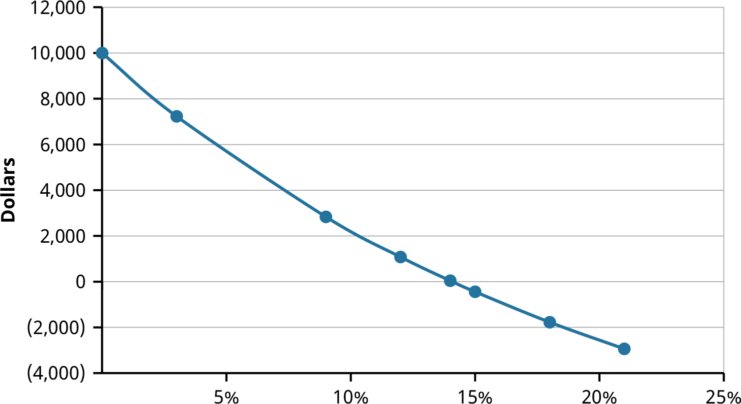
To construct an NPV profile for Sam’s, select several discount rates and compute the NPV for the embroidery machine project using each of those discount rates. Table 16.6 below shows the NPV for several discount rates. Notice that if the discount rate is zero, the NPV is simply the sum of the cash flows. As the discount rate becomes larger, the NPV falls and eventually becomes negative.
The information in Table 16.6 is presented in a graph in Figure 16.2. We can see that the graph crosses the horizontal axis at about 14%. To the left, or at lower discount rates, the NPV is positive. If you are confident that the firm’s cost of attracting funds is less than 14%, the company should accept the project. If the cost of capital is more than 14%, however, the NPV is negative, and the company should reject the project.
|
0% |
|
|
3% |
7,231 |
|
9% |
2,836 |
|
12% |
1,081 |
|
14% |
42 |
|
15% |
(442) |
|
18% |
(1,773) |
|
21% |
(2,939) |
Table 16.6 NPV for Various Discount Rates
16.3
Internal Rate of Return (IRR) Method
Learning Outcomes
By the end of this section, you will be able to:
- Define internal rate of return (IRR).
- Calculate internal rate of return.
- List advantages and disadvantages of using the internal rate of return method.
Internal Rate of Return (IRR) Calculation


 The internal rate of return (IRR) is the discount rate that sets the present value of the cash inflows equal to the present value of the cash outflows. In considering whether Sam’s Sporting Goods should purchase the embroidery machine, the IRR method approaches the time value of money problem from a slightly different angle. Instead of using the company’s cost of attracting funds for the discount rate and solving for NPV, as we did in the first NPV equation, we set NPV equal to zero and solve for the discount rate to find the IRR:


The IRR is the discount rate at which the NPV profile graph crosses the horizontal axis. If the IRR is greater than the cost of capital, a project should be accepted. If the IRR is less than the cost of capital, a project should be rejected. The NPV profile graph for the embroidery machine crossed the horizontal axis at 14%. Therefore, if Sam’s Sporting Goods can attract capital for less than 14%, the IRR exceeds the cost of capital and the embroidery machine should be purchased. However, if it costs Sam’s more than 14% to attract capital, the embroidery machine should not be purchased.
In other words, a company wants to accept projects that have an IRR that exceed the company’s cost of attracting funds. The cash flow from these projects will be great enough to cover the cost of attracting money from investors in addition to the other costs of the project. A company should reject any project that has an IRR less than the company’s cost of attracting funds; the cash flows from such a project are not enough to compensate the investors for the use of their funds.
Calculating IRR without a financial calculator is an arduous, time-consuming process that requires trial and error to find the discount rate that makes NPV exactly equal zero. Your calculator uses the same type of trial- and-error iterative process, but because it uses an automated process, it can do so much more quickly than you can. A problem that might require 30 minutes of detailed mathematical calculations by hand can be
completed in a matter of seconds with the assistance of a financial calculator.
All the information your calculator needs to calculate IRR is the value of each cash flow and the time period in which it occurs. To calculate IRR, begin by entering the cash flows for the project, just as you do for the NPV calculation (see Table 16.7). After these cash flows are entered, simply compute IRR in the final step.
Step1234Description Select cash flow worksheet Clear the cash flow worksheet Enter initial cash flowEnter cash flow for the first yearEnterCFCF02ND [CLR WORK] CF0DisplayXXXX016000 +/- ENTER CF0 = -16,000.00↓↓2000 ENTER5Enter cash flow for the second year ↓↓4000 ENTER6Enter cash flow for the third year7Enter cash flow for the fourth year8Enter cash flow for the fifth year9Enter cash flow for the sixth year↓↓↓↓↓↓↓↓5000 ENTER5000 ENTER5000 ENTER5000 ENTER10 Compute IRRIRR CPTC01 =2,000.00F01 =1.0C02 =4,000.00F02 =1.0C03 =5,000.00F03 =1.0C04 =5,000.00F04 =1.0C05 =5,000.00F05 =1.0C06 =5,000.00F06 =1.0IRR =14.09
Table 16.7 Calculator Steps for IRR
Advantages
The primary advantage of using the IRR method is that it is easy to interpret and explain. Investors like to speak in terms of annual percentage returns when evaluating investment possibilities.
Disadvantages
One disadvantage of using IRR is that it can be tedious to calculate. We knew the IRR was about 14% for the embroidery machine project because we had previously calculated the NPV for several discount rates. The IRR is about, but not exactly, 14%, because NPV is not exactly equal to zero (just very close to zero) when we use 14% as the discount rate. Before the prevalence of financial calculators and spreadsheets, calculating the exact IRR was difficult and time-consuming. With today’s technology, this is no longer a major consideration. Later in this chapter, we will look at how to use a spreadsheet to do these calculations.
No Single Mathematical Solution. Another disadvantage of using the IRR method is that there may not be a single mathematical solution to an IRR problem. This can happen when negative cash flows occur in more than one period in the project. Suppose your company is considering building a facility for an upcoming Olympic competition. The construction cost would be $350 million. The facility would be used for one year and generate cash inflows of $950 million. Then, the following year, your company would be required to convert the facility into a public park area for the city, which is expected to cost $620 million. Placing these cash flows in a timeline results in the following (Table 16.8):
|
0 |
1 |
2 |
|
|
Cash Flow ($Millions) |
(350) |
950 |
(620) |
Table 16.8
The NPV profile for this project looks like Figure 16.3. The NPV is negative at low interest rates, becomes positive at higher interest rates, and then turns negative again as the interest rate continues to rise. Because the NPV profile line crosses the horizontal axis twice, there are two IRRs. In other words, there are two interest rates at which NPV equals zero.
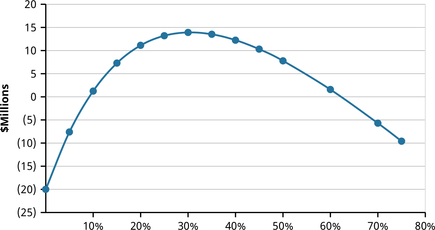
Figure 16.3 NPV Profile Graph for a Project with Two IRRs
Reinvestment Rate Assumption. The IRR assumes that the cash flows are reinvested at the internal rate of return when they are received. This is a disadvantage of the IRR method. The firm may not be able to find any other projects with returns equal to a high-IRR project, so the company may not be able to reinvest at the IRR.
The reinvestment rate assumption becomes problematic when a company has several acceptable projects and is attempting to rank the projects. We will look more closely at the issues that can arise when considering mutually exclusive projects later in this chapter. If a company is simply deciding whether to accept a single project, the reinvestment assumption limitation is not relevant.
Overlooking Differences in Scale. Another disadvantage of using the IRR method to choose among various acceptable projects is that it ignores differences in scale. The IRR converts the cash flows to percentages and ignores differences in the size or scale of projects. Issues that occur when comparing projects of different scales are covered later in this chapter.
16.4
Alternative Methods
Learning Outcomes
By the end of this section, you will be able to:
- Calculate profitability index.
- Calculate discounted payback period.
- Calculate modified internal rate of return.
Profitability Index (PI)
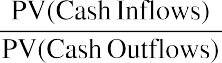
The profitability index (PI) uses the same inputs as the NPV calculation, but it converts the results to a ratio. The numerator is the present value of the benefits of doing a project. The denominator is the present value of
the cost of doing the project. The formula for calculating PI is

For the embroidery machine project that Sam’s Sporting Goods is considering, the PI would be calculated as

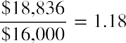
The numerator of the PI formula is the benefit of the project, and the denominator is the cost of the project. Thus, the PI is the benefit relative to the cost. When NPV is greater than zero, PI will be greater than 1. When NPV is less than zero, PI will be less than 1. Therefore, the decision criterion using the PI method is to accept a project if the PI is greater than 1 and reject a project if the PI is less than 1.
Note that the NPV method and the PI method of project evaluation will always provide the same answer to the accept-or-reject question. The advantage of using the PI method is that it is helpful in ranking projects from best to worst. Issues that arise when ranking projects are discussed later in this chapter.
Discounted Payback Period
The payback period method provides a fast, simple approach to evaluating a project, but it suffers from the fact that it ignores the time value of money. The discounted payback period method addresses this flaw by discounting cash flows using the company’s cost of funds and then using these discounted values to determine the payback period.
Consider Sam’s Sporting Goods’ decision regarding whether to purchase an embroidery machine. The expected cash flows and their values when discounted using the company’s 9% cost of funds are shown in Table 16.9. Earlier, we calculated the project’s payback period as four years; that is how long it would take the company to recover all of the cash that it would spend on the project. Remember, however, that the payback period does not consider the company’s cost of funds, so it underestimates the true breakeven time period.
|
0 |
1 |
2 |
3 |
4 |
5 |
6 |
|
|
Cash Flow ($) |
(16,000.00) |
2,000.00 |
4,000.00 |
5,000.00 |
5,000.00 |
5,000.00 |
5,000.00 |
|
Discounted Cash Flow ($) |
(16,000) |
1,834.86 |
3,366.72 |
3,860.92 |
3,542.13 |
3,249.66 |
2,981.34 |
|
Cumulative Discounted Cash Flow ($) |
(16,000.00) |
(14,165.14) |
(10,798.42) |
(6,937.50) |
(3,395.37) |
(145.72) |
2,835.62 |
Table 16.9
When the cash flows are appropriately discounted, the project still has not broken even by the end of year 5. The discounted payback period would be 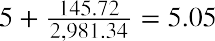 years. This adjusted calculation addresses the payback period method’s flaw of not considering the time value of money, but managers are still confronted with the other disadvantages. No objective criterion for acceptance or rejection exists because of the lack of a
theoretical underpinning for what is an acceptable payback period length. The discounted payback period ignores any cash flows after breakeven occurs; this is a serious drawback, especially when comparing mutually exclusive projects.
Modified Internal Rate of Return (MIRR)
Financial analysts have developed an alternative evaluation technique that is similar to the IRR but modified in an attempt to address some of the weakness of the IRR method. This modified internal rate of return (MIRR) is calculated using the following steps:
- Find the present value of all of the cash outflows using the firm’s cost of attracting capital as the discount
rate.
- Find the future value of all cash inflows using the firm’s cost of attracting capital as the discount rate. All cash inflows are compounded to the point in time at which the last cash inflow will be received. The sum of the future value of cash inflows is known as the project terminal value.
- Compute the yield that sets the future value of the inflows equal to the present value of the outflows. This yield is the modified internal rate of return.
For our embroidery machine project, the MIRR would be calculated as shown in Table 16.10:
|
0 |
1 |
2 |
3 |
4 |
5 |
6 |
|
|
Cash Flow ($) |
(16,000.00) |
2,000.00 |
4,000.00 |
5,000.00 |
5,000.00 |
5,000.00 |
5,000.00 |
|
|
|
|
|
|
|
|
3,077.25 |
|
|
|
|
|
|
|
|
5,646.33 |
|
|
|
|
|
|
|
|
6,475.15 |
|
|
|
|
|
|
|
|
5,940.50 |
|
|
|
|
|
|
|
|
5,450.00 |
|
|
|
|
|
|
|
Terminal Value |
$31,595.22 |
Table 16.10
- The only cash outflow is the $16,000 at time period 0.
- The future value of each of the six expected cash inflows is calculated using the company’s 9% cost of attracting capital. Each of the cash flows is translated to its value in time period 6, the time period of the final cash inflow. The sum of the future value of these six cash flows is $31,595.22. Thus, the terminal value is $31,595.22
- The interest rate that equates the present value of the outflows, $16,000, to the terminal value of


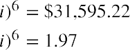 $31,595.22 six years later is found using the formula


The MIRR solves the reinvestment rate assumption problem of the IRR method because all cash flows are compounded at the cost of capital. In addition, solving for MIRR will result in only one solution, unlike the IRR, which may have multiple mathematical solutions. However, the MIRR method, like the IRR method, suffers from the limitation that it does not distinguish between large-scale and small-scale projects. Because of this limitation, the MIRR cannot be used to rank projects; it can only be used to make accept-or-reject decisions.
16.5
Choosing between Projects
Learning Outcomes
By the end of this section, you will be able to:
- Choose between mutually exclusive projects.
- Compare projects with different lives.
- Compare projects of different scales.
- Rank projects when resources are limited.
So far, we have considered methods for deciding to accept or to reject a single stand-alone project. Sometimes, managers must make decisions regarding which of two projects to accept, or a company might be faced with a number of good, acceptable projects and have to decide which of those projects to take on during
the current year.
Choosing between Mutually Exclusive Projects
Earlier in this chapter, we saw that the embroidery machine that Sam’s Sporting Goods was considering had a positive NPV, making it a project that Sam’s should accept. However, another, more expensive embroidery machine may be available that is able to make more stitches per minute. Although the initial cost of this heavy- duty machine is higher, it would allow Sam’s to embroider and sell more items each year, generating more revenue. The two embroidery machines are mutually exclusive projects. Mutually exclusive projects compete with one another; purchasing one embroidery machine excludes Sam’s from purchasing the other embroidery machine.
Table 16.11 shows the cash outflow and inflows expected from the original embroidery machine considered as well as the heavy-duty machine. The heavy-duty machine costs $25,000, but it will generate more cash inflows in years 3 through 6. Both machines have a positive NPV, leading to decisions to accept the projects. Also, both machines have an IRR exceeding the company’s 9% cost of raising capital, also leading to decisions to accept the projects.
When considered by themselves, each of the machines is a good project for Sam’s to pursue. The question the managers face is which is the better of the two projects. When faced with this type of decision, the rule is to take the project with the highest NPV. Remember that the goal is to choose projects that add value to the company. Because the NPV of a project is the estimate of how much value it will create, choosing the project with the higher NPV is choosing the project that will create the greater value.
|
0 |
1 |
2 |
3 |
4 |
5 |
6 |
NPV |
IRR |
|
|
Regular Machine ($) |
(16,000) |
2,000 |
4,000 |
5,000 |
5,000 |
5,000 |
5,000 |
2,835.62 |
14.10% |
|
Heavy-Duty Machine ($) |
(25,000) |
2,000 |
4,000 |
8,000 |
9,000 |
9,000 |
9,000 |
3,970.67 |
13.20% |
Table 16.11
LINK TO LEARNINGOlympic Project EconomicsThe investment analysis procedures used by companies are also used by government entities when evaluating projects. Olympic host cities receive direct revenues from broadcast rights, ticket sales, and licensing agreements. The cities also expect indirect benefits from increased tourism, including increased employment and higher tax revenues. These benefits come after the city makes a major investment in infrastructure, spending money on stadiums, housing, and transportation. The investment in infrastructure for the 2014 Winter Olympics in Sochi, Russia, was over $50 billion.2 Why do you think the infrastructure investment for these games was so much higher than the amount spent by cities hosting previous games? If your city were discussing the possibility of bidding to be an Olympic host city, what would you suggest it consider when evaluating the opportunity? Check out this article (https://openstax.org/r/this-article) for more information.
Choosing between Projects with Different Lives
Suppose you are considering starting an ice-cream truck business. You find that you can purchase a used truck for $50,000. You estimate that the truck will last for three years, and you will be able to sell enough ice cream
2 David Filipov. “Russia Spent $50 Billion on the Sochi Olympics. It Might Actually Have Been Worth It.” Washington Post, November 15, 2017. https://www.washingtonpost.com/world/europe/that-sochi-olympic-boondoggle-russians-say-all-the-investment-is- paying-off/2017/11/13/65014bd0-b82c-11e7-9b93-b97043e57a22_story.html
treats to generate a cash inflow of $40,000 during each of those years. Your cost of capital is 10%. The positive NPV of $49,474 for the project makes this an acceptable project.
Another ice-cream truck is also for sale for $50,000. This truck is smaller and will not be able to hold as many frozen treats. However, the truck is newer, with lower mileage, and you estimate that you can use it for six years. This newer truck will allow you to generate a cash inflow of $30,000 each year for the next six years. The NPV of the newer truck is $80,658.
Because both trucks are acceptable projects but you can only drive one truck at a time, you must choose which truck to purchase. At first, it may be tempting to purchase the newer, lower-mileage truck because of its higher NPV. Unfortunately, when comparing two projects that have different lives, a decision cannot be made simply by comparing the NPVs. Although the ice-cream truck with the six-year life span has a much higher NPV than the larger truck, it consumes your resources for a long time.
There are two methods for comparing projects with different lives. Both assume that when the short-life project concludes, another, similar project will be available.
Replacement Chain Approach
With the replacement chain approach, as many short-life projects as necessary are strung together to equal the life of the long-life project. You can purchase the newer, lower-mileage ice-cream truck and run your business for six years. To make a comparison, you assume that if you purchase the larger truck that will last for three years, you will be able to repeat the same project, purchasing another larger truck that will last for the next three years. In essence, you are comparing a six-year project with two consecutive three-year projects so that both options will generate cash inflows for six years. Your timeline for the projects (comparing an older, larger truck with a newer, lower-mileage truck) will look like Table 16.12:
|
0 |
1 |
2 |
3 |
4 |
5 |
6 |
|
|
Older Truck ($) |
($50,000) |
40,000 |
40,000 |
40,000 |
40,000 |
40,000 |
40,000 |
|
Older Truck ($) |
|
|
|
(50,000) |
|
|
|
|
|
|
|
|
|
|
|
|
|
Newer Truck ($) |
(50,000) |
30,000 |
30,000 |
30,000 |
30,000 |
30,000 |
30,000 |
Table 16.12
The present values of all of the cash inflows and outflows from purchasing two of the older, larger trucks consecutively are added together to find the NPV of that alternative. The NPV of this alternative is $86,645, which is higher than the NPV of $80,658 of the newer truck, as shown in Table 16.13:
|
0 |
1 |
2 |
3 |
4 |
5 |
6 |
|
|
Older Truck ($) |
|
40,000 |
40,000 |
40,000 |
40,000 |
40,000 |
40,000 |
|
Older Truck ($) |
|
|
|
(50,000) |
|
|
|
|
Net Present Value |
(50,000) |
36,363.64 |
33,057.85 |
(7,513.15) |
27,320.54 |
24,836.85 |
22,578.96 |

Table 16.13
When using the replacement chain approach, the short-term project is repeated any number of times to equal the length of the longer-term project. If one project is 5 years and another is 20 years, the short one is
repeated four times. This method can become tedious when the length of the longer project is not a multiple of the shorter project. For example, when choosing between a five-year project and a seven-year project, the short one would have to be duplicated seven times and the long project would have to be repeated five times to get to a common length of 35 years for the two projects.
Equal Annuity Approach
The equal annuity approach assumes that both the short-term and the long-term projects can be repeated forever. This approach involves the following steps:
Step 1: Find the NPV of each of the projects.
- The NPV of the larger, older ice-cream truck is $49,474.
- The NPV of the smaller, newer ice-cream truck is $80,658.
Step 2: Find the annuity that has the same present value as the NPV and the same number of periods as the project.
- For the larger, older ice-cream truck, we want to find the three-year annuity that would have a present value of $49,474 when using a 10% discount rate. This is $19,894.
- For the smaller, newer ice-cream truck, we want to find the six-year annuity that would have a present value of $80,658 when using a 10% discount rate. This is $18,520.
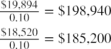 Step 3: Assume that these projects, or similar projects, can be repeated over and over and that these annuities will continue forever. Calculate the present value of these annuities continuing forever using the perpetuity formula.


We again find that the older, larger truck is preferred to the newer, smaller truck.
These methods correct for unequal lives, but managers need to be aware that some unavoidable issues come up when these adjustments are made. Both the replacement chain and equal annuity approaches assume that projects can be replicated with identical projects in the future. It is important to note that this is not always a reasonable assumption; these replacement projects may not exist. Estimating cash flows from potential projects is prone to errors, as we will discuss in Financial Forecasting these errors are compounded and become more significant as projects are expected to be repeated. Inflation and changing market conditions are likely to result in cash flows varying in the future from our predictions, and as we go further into the future, these changes are potentially greater.
Choosing Projects When Resources Are Limited
Choosing positive NPV projects adds value to a company. Although we often assume that the company will choose to pursue all positive NPV projects, in reality, managers often face a budget that restricts the amount of capital that they may invest in a given time period. Thus, managers are forced to choose among several positive NPV projects. The goal is to maximize the total NPV of the firm’s projects while remaining within budget constraints.
LINK TO LEARNINGProfitability IndexManagers should reject any project with a negative NPV. When managers find themselves with an array of projects with a positive NPV, the profitability index can be used to choose among those projects. To learn
more, watch this video about how a company might use the profitability index (https://openstax.org/r/ might-use).
P
For example, suppose Southwest Manufacturing is considering the seven projects displayed in Table 16.14. Each of the projects has a positive NPV and would add value to the company. The firm has a budget of $200 million to put toward new projects in the upcoming year. Doing all seven of the projects would require initial investments totaling $430 million. Thus, although all of the projects are good projects, Southwest Manufacturing cannot fund them all in the upcoming year and must choose among these projects. Southwest Manufacturing could choose the combination of Projects A and D; the combination of Projects B, C, and E; or several other combinations of projects and exhaust its $200 million investment budget.
Table 16.14 Projects Being Considered by Southwest Manufacturing
ProjectNPV ($Millions)Initial Investment($Millions)ProfitabilityIndexCumulative Investment Required($Millions)
To decide which combination results in the largest added NPV for the company, rank the projects based on their profitability index, as is done in Table 16.15. Projects A, E, and F should be chosen, as they have the highest profitability indexes. Because those three projects require a cumulative investment of $200 million, none of the remaining projects can be undertaken at the present time. Doing those three projects will add $78 million in NPV to the firm. Out of this set of choices, there is no combination of projects that is affordable given Southwest Manufacturing’s budget that would add more than $78 million in NPV.
|
60 |
150 |
1.40 |
150 |
|
|
E |
11 |
30 |
1.37 |
180 |
|
F |
7 |
20 |
1.35 |
200 |
|
D |
15 |
50 |
1.30 |
250 |
|
B |
25 |
100 |
1.25 |
350 |
|
G |
2 |
10 |
1.20 |
360 |
|
C |
10 |
70 |
1.14 |
430 |
Table 16.15 Projects Ranked by Profitability Index
Notice that when choices must be made among projects, the decision cannot be made by simply ranking the projects from highest to lowest NPV. Project D has an NPV of $15 million, which is higher than both the $11 million of Project E and the $7 million of Project F. However, Project D requires $50 million for an initial
investment. For the same $50 million of investment funds, Southwest Manufacturer can accept both Projects E and F for a total NPV of $18 million. Investment capital is a scare resource for this company. By ranking projects based on their profitability index, the company is able to determine the best way to allocate its scarce capital for the largest potential increase in NPV.
CONCEPTS IN PRACTICE
Capital Budgeting Challenges
Although the basic techniques of project evaluation are straightforward, real-world capital budgeting decisions are complex and multifaceted. The goal of capital budgeting is to choose the projects that will bring the most value to the shareholders of the company. The NPV rule provides a clear, concise criterion for which projects will bring value to the shareholders. It is important to remember, however, that all of the project valuation calculations are based on projected cash flows. These projected cash flows are estimates, based on the best educated guesses that a company makes about its business opportunities over the next few years. Because no company has a crystal ball that can predict the future, its calculation of NPV is an estimate of what it expects.
Think, for example, of an oil company deciding whether to drill for oil. The project will require expenditures on equipment, land, and other items. The cash inflows will depend on the likelihood of oil being found, the quantity of oil produced by the well, and the price at which the oil can be sold. If a company estimates that oil will sell for $100 per barrel during the next few years, the project will have a much higher NPV than if the company estimates that oil will sell for only $50 per barrel.
A project that has a positive NPV and is accepted when a company is planning how to allocate its capital toward investments may end up being a bad project that the company wishes it had avoided if the future is much different from what it projected. Managers must stay attuned to economic developments and reevaluate capital budgeting decisions when significant changes occur. In spring 2020, managers around the globe were faced with a dramatically changing economic environment amid a pandemic. Oil companies, for example, saw oil prices drop from over $50 per barrel at the beginning of March to under $15 per barrel by the end of April.
LINK TO LEARNINGReducing Capital SpendingIn June 2020, McKinsey & Company looked at major companies around the world that were reducing their capital expenditures in the face of the COVID-19 pandemic. These companies were cutting their capital budgets by 10% to 80% from their originally planned levels for 2020. Reductions were especially large in the oil and gas industry, as companies found their revenue projections, and thus the NPV of their planned projects, falling dramatically. In addition, companies found themselves needing to free up cash; with more limited cash resources, fewer positive NPV projects could be accepted and funded.3 Due to the COVID-19 pandemic, many CFOs were challenged to stabilize their corporate cash flows. This article explains how quickly reducing capital spending (https://openstax.org/r/quickly-reducing), which is usually a quick enough fix, was able to help.
3 Tom Brinded, Zak Cutler, Erikhans Kok, and Prakash Parbhoo. “Resetting Capital Spending in the Wake of COVID-19.” McKinsey & Company. June 25, 2020. https://www.mckinsey.com/business-functions/operations/our-insights/resetting-capital-spending-in-the- wake-of-covid-19
16.6
Using Excel to Make Company Investment Decisions
Learning Outcomes
By the end of this section, you will be able to:
- Calculate NPV using Excel.
- Calculate IRR using Excel.
- Create an NPV profile using Excel.
A Microsoft Excel spreadsheet provides an alternative to using a financial calculator to automate the arithmetic necessary to calculate NPV and IRR. An advantage of using Excel is that you can quickly change any assumptions or numbers in your problem and recalculate NPV or IRR based on that updated information.
Excel is a versatile tool with more than one way to set up most problems. We will consider a couple of straightforward examples of using Excel to calculate NPV and IRR.
Suppose your company is considering a project that will cost $30,000 this year. The cash inflow from this project is expected to be $6,000 next year and $8,000 the following year. The cash inflow is expected to increase by $2,000 yearly, resulting in a cash inflow of $18,000 in year 7, the final year of the project. You know that your company’s cost of funds is 9%. Your company would like to evaluate this project.
Calculating NPV Using Excel
To calculate NPV using Excel, you would begin by placing each year’s expected cash flows in a sheet, as in row 5 in Figure 16.4. One approach to calculating NPV is to use the formula for discounting future cash flows, as is shown in row 6.
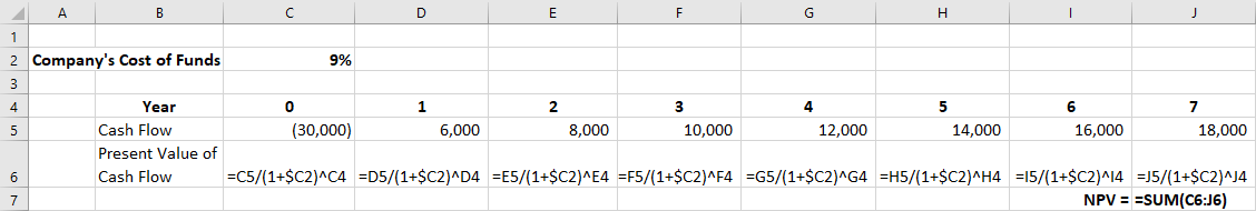
Figure 16.4 Inserting Present Cash Flows Using Excel ($ except Cost of Funds)
Figure 16.5 shows the present value of each year’s cash flow resulting from the formula. The NPV is then calculated by summing the present values of the cash flows.

Download the spreadsheet file (https://openstax.org/r/spreadsheet-file) containing key Chapter 16 Excel exhibits.
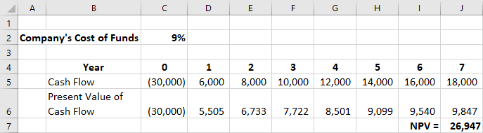
Figure 16.5 NPV Calculated by Summing Present Values of Cash Flows ($ except Cost of Funds)
Alternatively, Excel is programmed with financial functions, including a calculation for NPV. The NPV formula is shown in cell J7 in Figure 16.6 below. However, it is important to pay attention to how Excel defines NPV. The Excel NPV function calculates the sum of the present values of the cash flows occurring from period 1 through the end of the project using the designated discount rate, but it fails to include the initial investment at time
period zero at the beginning of the project. The NPV function in cell J6 will return $56,947 for this project. You must subtract the initial cash outflow of $30,000 that occurs at time 0 to get the NPV of $26,947 for the project.
When entering the Excel-programmed NPV function, you must remember to include references only to the cells that contain cash flows from year 1 to the end of the project. Then, subtract the initial investment of year 0 to calculate NPV according to the standard definition of NPV—the present values of the cash inflows minus the present value of the cash outflow. Note: Because of the nonstandard use of the term NPV by Excel, many users prefer to use the method described above rather than this predefined function.
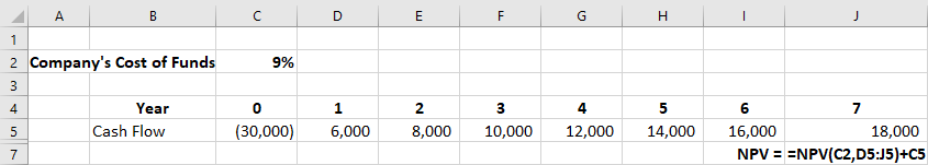
Figure 16.6 NPV Formula ($ except IRR/Cost of Funds)
Calculating IRR Using Excel
Excel also provide a function for calculating IRR. This function is shown in Figure 16.7, cell J8. The IRR function properly uses all the project’s cash flows, including the initial cash outflow at time 0, in its calculation, unlike the NPV function. This function will correctly return the IRR of 27.7% for the project. Figure 16.8 shows the completed spreadsheet.
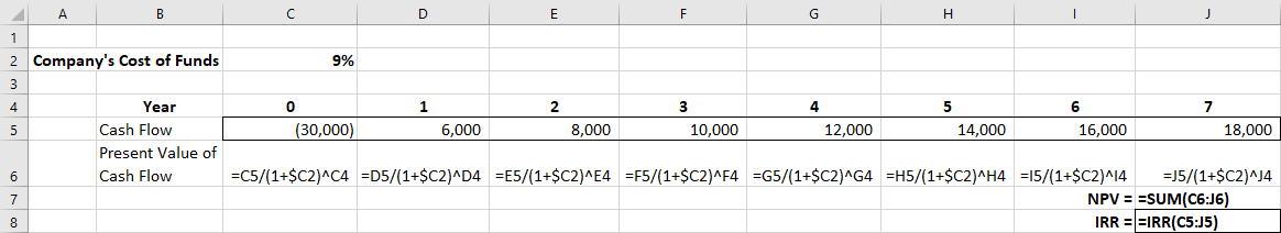
Figure 16.7 Function for Calculating IRR ($ except IRR/Cost of Funds)
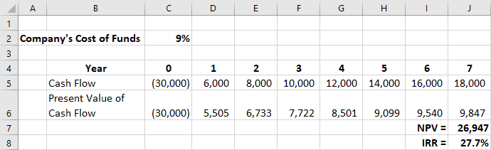
Figure 16.8 Final Spreadsheet ($ except IRR/Cost of Funds)
Using Excel to Create an NPV Profile
Firms often do not know exactly what their cost of attracting capital is, so they must use estimates in their decision-making. Also, the cost of attracting capital can change with economic and market conditions.
Especially if markets are volatile, a company may use an NPV profile to see how sensitive their decisions are to changes in financing costs. Excel simplifies the creation of an NPV profile.
Middleton Manufacturing is considering installing solar panels to heat water and provide lighting throughout its plant. To do so will cost the company $800,000 this year. However, this upgrade will save the company an estimated $150,000 in electrical costs each year for the next 10 years. Constructing an NPV profile of this project will allow Middleton to see how the NPV of the project changes with the cost of attracting funds.
First, the project cash flows must be placed in an Excel spreadsheet, as is shown in cells D2 through N2 in Figure 16.9. The company’s cost of funds is placed in cell B1; begin by putting in 10% for this rate. Next, the formula for NPV is placed in cell B6; cell B6 shows the NPV of the cash flows in cells D2 through N2, using the rate that is in cell B1.
For reference, compute IRR in cell B4. Calculating IRR is not necessary for creating the NPV profile. However, it gives a good reference point. Remember that if the IRR of a project is greater than the firm’s cost of attracting capital, then the NPV will be positive; if the IRR of a project is less than the firm’s cost of attracting capital, then the NPV will be negative.
An NPV profile is created by calculating the NPV of the project for a variety of possible costs of attracting capital. In other words, you want to calculate NPV using the project cash flows in cells D2 through N2, using a variety of discount rates in cell B1. This is accomplished by using the Excel data table function. The data table function shows how the outcome of an Excel formula changes when one of the cells in the spreadsheet changes. In this instance, you want to determine how the value of the NPV formula (cell B6) changes when the discount rate (cell B1) changes.
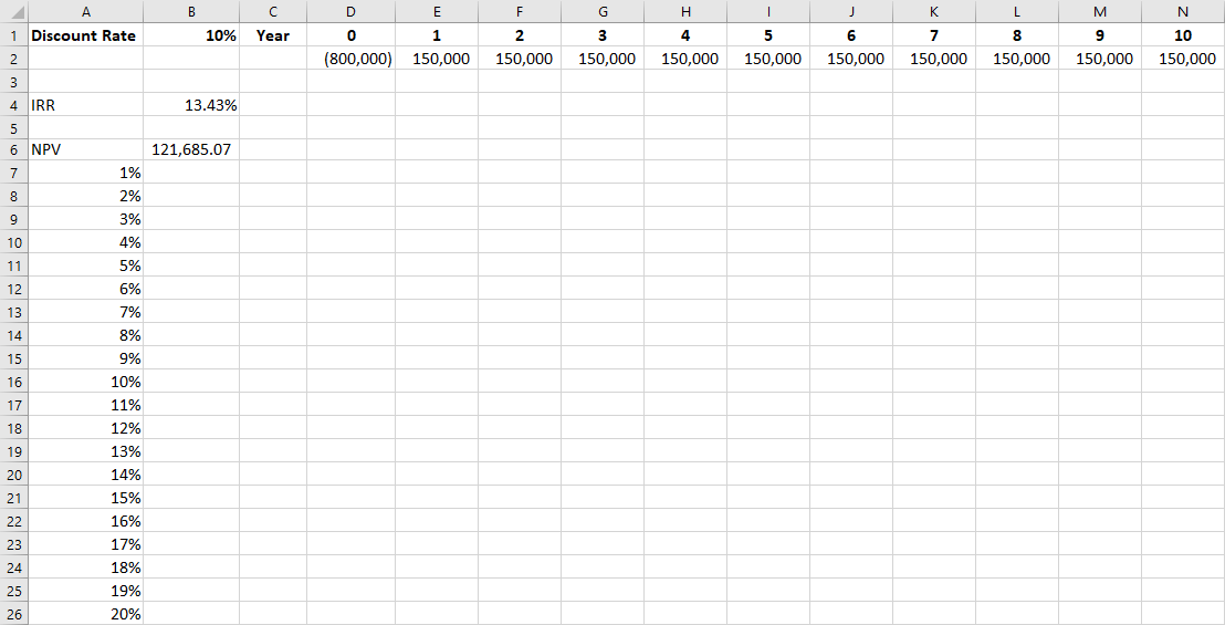
Figure 16.9 Project Cash Flows Inserted into Excel
To do this, enter the range of interest rates that you want to consider down a column, beginning in cell A7. This example shows rates from 1% to 20% entered in cells A7 through A26. Your Excel file should now look like the screenshot in Figure 16.9.
Next, highlight the cells containing the NPV calculation and the range of discount rates. Thus, you will highlight cells A6 through A26 and B6 through B26 (see Figure 16.10). Click Data at the top of the Excel menu so that you see the What-If Analysis feature. Choose Data Table. Because the various discount rates you want to use are in a column, use the “Column input cell” option. Enter “B1” in this box. You are telling Excel to calculate NPV using each of the numbers in this column as the cost of attracting funds in cell B1. Click OK.
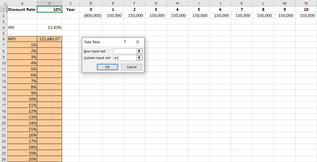
Figure 16.10 Creating a Data Table in Excel
After clicking OK, the cells in column B next to the list of various discount rates will fill with the NPVs corresponding to each of the rates. This is shown in Figure 16.11.
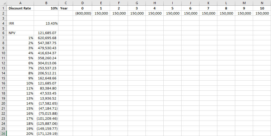
Figure 16.11 NPV Calculated for Various Discount Rates
Now that the various NPVs are calculated, you can create the NPV profile graph. To create the graph, begin by highlighting the discount rates and NPVs that are in cells A7 through A26 and B7 through B26. Next, go to the Insert tab in the menu at the top of Excel. Several different chart options will be available; choose Scatter. You will end up with a chart that looks like the one in Figure 16.12. You can customize the chart by renaming it, labeling the axes, and making other cosmetic changes if you like.
You will notice that the NPV profile crosses the x-axis between 13% and 14%; remember that the NPV will be zero when the discount rate that is used to calculate the NPV is equal to the project’s IRR, which we previously calculated to be 13.43%. If the firm’s cost of raising funds is lower than 13.43%, the NPV profile shows that the project has a positive NPV, and the project should be accepted. Conversely, if the firm’s cost of raising funds is greater than 13.43%, the NPV of this project will be negative, and the project should not be accepted.
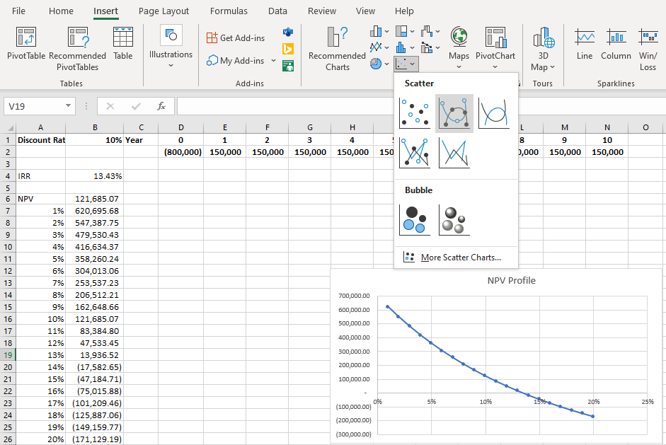
Figure 16.12 NPV Profile Created Using Excel
Middleton Manufacturing can use this NPV profile to evaluate its solar panel installation project. If the managers think that the cost of attracting funds for the company is 10%, then the project has a positive NPV of
$121,685 and the company should install the panels. The NPV profile shows that if the managers are underestimating the cost of funds even by 30% and it will really cost Middleton 13% to attract funds, the project is still a good project. The cost of attracting funds would have to be higher than 13.43% for the solar panel project to be rejected.
 Summary
Payback Period Method
The payback period is the simplest project evaluation method. It is the time it takes the company to recoup its initial investment. Its usefulness is limited, however, because it ignores the time value of money.
Net Present Value (NPV) Method
Net present value (NPV) is calculated by subtracting the present value of a project’s cash outflows from the present value of the project’s cash inflows. A project should be accepted if its NPV is positive and rejected if its NPV is negative.
Internal Rate of Return (IRR) Method
The internal rate of return (IRR) of a project is the discount rate that sets the present value of a project’s cash inflows exactly equal to the present value of the project’s cash outflows. A project should be accepted if its IRR is greater than the firm’s cost of attracting capital.
Alternative Methods
The discounted payback period uses the time value of money to discount future cash flows to see how long it will be before the initial investment of a project is recovered. MIRR provides a variation on IRR in which all cash flows are compounded using the cost of capital, resolving the reinvestment rate assumption problem of the IRR method; unlike IRR, which may have multiple mathematical solutions, MIRR will result in one solution. The profitability index is calculated as the NPV of the project divided by the initial cost of the project.
Choosing between Projects
Firms may need to choose among a variety of good projects. The projects may have different lives or be differently sized projects that require different amounts of resources. By choosing projects with the highest profitability index, companies can take on the projects that will lead to the greatest increase in value for the company.
Using Excel to Make Company Investment Decisions
Excel spreadsheets provide a way to easily calculate the NPV and IRR of a project. Using Excel to create an NPV profile allows a company to see how much its estimates of the cost of raising funds can err from the true cost and have the project still be an acceptable project.
 Key Terms
capital budgeting the process a business follows to evaluate potential major projects or investments
discounted payback period the length of time it will take for the present value of the future cash inflows of a project to equal the initial cost of the investment
equal annuity approach a method of comparing projects of different lives by assuming that the projects can be repeated forever
internal rate of return (IRR) the discount rate that sets the NPV of a project equal to zero
modified internal rate of return (MIRR) the yield that sets the future value of the cash inflows of a project equal to the present value of the cash outflows of the project
mutually exclusive projects projects that compete against each other so that when one project is chosen, the other project cannot be done
net present value (NPV) the present value of the cash inflows of a project minus the present value of the cash outflows of the project
payback period the length of time it will take for a company to make enough money from an investment to recover the initial cost of the investment
profitability index (PI) the present value of cash inflows divided by the present value of cash outflows
replacement chain approach a method of comparing projects of differing lives by repeating shorter projects multiple times until they reach the lifetime of the longest project