12 Lesson 7 Risk and Return
Having finished her college degree and embarked on her career, Maria is now contemplating her financial future. She is considering how she might invest some of her hard-earned money. As a short-term goal, she wants to build an emergency fund so that she could cover her expenses for six months if she became ill or injured and had to take time off of work. She would also like to save money for a down payment on a home and to purchase new furniture. Although she is not yet 30 years old, Maria also knows that it is prudent to begin saving for retirement.
What should she do with her savings? Maria has some friends who have told her how successful they have been investing in stocks. Bart bragged about doubling his money in just over a year when he purchased Facebook stock, and Tiffany quickly tripled her money when she purchased shares in Netflix. But Maria also knows that her uncle lost a significant amount of money when his Boeing stock dropped from over $300 per share to under $150 within a couple of months at the beginning of 2020. Just how risky would it be to invest in stocks? What type of return might Maria expect? Are there strategies she could follow that would allow her to avoid her uncle’s fate?
 15.1
15.1
Risk and Return to an Individual Asset
Learning Outcomes
By the end of this section, you will be able to:
- Compute the realized return from an individual investment.
- Compute the average return and volatility of returns from historical data.
- Describe firm-specific risk.
Measuring Historical Returns
Risk and return are often referred to as the two Rs of finance. Investors are interested in both risk and return because understanding one without the other is really meaningless. In terms of investment, the concept of return is fairly straightforward; return is the benefit, or profit, the investor expects from an expenditure. It is the reward for investing—the reason an investment is made in the first place. However, no investment is a sure thing. The return may not be what the investor was expecting. This uncertainty about what the return will be is referred to as risk.
We begin by looking at how to measure both risk and return when considering an individual asset, such as one stock. If your grandparents bought 100 shares of Apple, Inc. stock for you when you were born, you are interested in knowing how well that investment has done. You may even want to compare how that investment has fared to how an investment in a different stock, perhaps Disney, would have done. You are interested in measuring the historical return.
Individual Investment Realized Return
The realized return of an investment is the total return that occurs over a particular time period. Suppose that you purchased a share of Target (TGT) at the beginning of January 2020 for $128.74. At the end of the year, you sold the stock for $176.53, which was $47.79 more than you paid for it. This increase in value is known as a capital gain. As the owner of the stock, you also received $2.68 in dividends during 2020. The total dollar return from your investment is calculated as


It is common to express investment returns in percentage terms rather than dollar terms. This allows you to answer the question “How much do I receive for each dollar invested?” so that you can compare investments of different sizes. The total percent return from your investment is

The dividend yield is calculated by dividing the dividends you received by the initial stock price. This calculation says that for each dollar invested in TGT in 2020, you received $0.0208 in dividends. The capital gain yield is the change in the stock price divided by the initial stock price. This calculation says that for each dollar invested in TGT in 2020, you received $0.3712 in capital gains. Your total percent return of 39.20% means that you made $0.392 for every dollar invested when your gains from both dividends and stock price appreciation are totaled together.
THINK IT THROUGHCalculating ReturnYou purchased 10 shares of 3M (MMM) stock in January 2020 for $175 per share, received dividends of $5.91
 per share, and sold the stock at the end of the year for $169.72 per share. Calculate your total dollar return, your dividend yield, your capital gain yield, and your total percent yield.Solution:Because you purchased 10 shares, you receivedin dividend income. You spentto purchase the stock, and you sold it forYour totaldollar return isYour dividend yield is, or 3.38%, and your capital gain yield isor 3.02%. Your total percent return isNotice that you sold MMM for a price lower than what you paid for it at the beginning of the year. Your capital gain is negative, or what is often referred to as a capital loss. Although the price fell, you still had apositive total dollar return because of the dividend income.
Of course, investors seldom purchase a stock and then sell it exactly one year later. Assume that you purchased shares of Facebook (FB) on June 1, 2020, for $228.50 per share and sold the shares three months later for $261.90. You received no dividends. In this case, your holding period percentage return is calculated as
This 14.62% is your return for a three-month holding period. To compare them to other investment opportunities, you need to express returns on a per-year, or annualized, basis. The holding period returned is converted to an effective annual rate (EAR) using the formula

where m is the number of holding periods in a year.
There are four three-month periods in a year. So, the EAR for this investment is


What happens if you own a stock for more than one year? Your holding period return would have occurred over a period longer than a year, but the process to calculate the EAR is the same. Suppose you purchased shares of FB in May 2015, when it was selling for $79.30 per share. You held the stock until May 2020, when you

sold it for $224.59. Your holding period percentage return would be  . You more
than tripled your money, but it took you five years to do so. Your EAR, which will be smaller than this five-year holding period return rate, is calculated as


Average Annual Returns


 Suppose that you purchased shares of Delta Airlines (DAL) at the beginning of 2011 for $11.19 and held the stock for 10 years before selling it for $40.21. You madeon your investment over a 10-year period. This is a 259.34% holding period return. The EAR for this investment is


To calculate the EAR using the above formula, the holding period return must first be calculated. The holding period return represents the percentage return earned over the entire time the investment is held. Then the holding period return is converted to an annual percentage rate using the formula.
You can also use the basic time value of money formula to calculate the EAR on an investment. In time value of money language, the initial price paid for the investment, $11.19, is the present value. The price the stock is sold for, $40.21, is the future value. It takes 10 years for the $11.19 to grow to $40.21. Using the time value of money will result in a calculation of


The EAR formula and the time value of money both result in a 13.65% annual return. Mathematically, the two formulas are the same; one is simply an algebraic rearrangement of the other.
If you earned 13.65% each year, compounded for 10 years, you would have converted your $11.19 per share investment to $40.21 per share. Of course, DAL stock did not increase by exactly 13.65% each year. The returns for DAL for each year are shown in Table 15.1. Some years, the return was much higher than 13.65%. In 2013, the return was almost 133%! Other years, the return was much lower than 13.65%; in fact, in the return was negative in four of the years.
|
|
|
Initial investment of 11.19 |
|
2011 |
−0.3579 |
7.19 |
|
2012 |
0.4672 |
10.54 |
|
2013 |
1.3261 |
24.52 |
|
2014 |
0.8053 |
44.27 |
|
2015 |
0.0405 |
46.06 |
|
2016 |
−0.0135 |
45.44 |
|
2017 |
0.1623 |
52.81 |
|
2018 |
−0.0866 |
48.24 |
|
2019 |
0.2038 |
58.07 |
|
2020 |
−0.3077 |
40.20 |
Table 15.1 Yearly Returns for DAL, 2011–2020:
Value of Initial Investment at Each Year End


Although an investment in DAL of $11.19 at the beginning of 2011 grew to $40.20 by the end of 2020, this growth was not consistent each year. The amount that the stock was worth at the end of each year is also shown in Table 15.1. During 2011, the return for DAL was −35.79%, resulting in the value of the investment falling to. The following year, 2012, the return for DAL was 46.72%. Therefore, the value of the investment was at the end of 2012. This process continues each year that the stock is held.
The compounded annual return derived from the EAR and time value of money formulas is also known as a
geometric average return. A geometric average return is calculated using the formula


where RN is the return for each year in the time period for which the average is calculated.
The calculation of the geometric average return for DAL is shown in the right column of Table 15.2. (The slight difference in the geometric average return of 13.64% from the 13.65% derived from the EAR and time value of money calculations is due to rounding errors.)
|
Return |
1 + Return |
|
|
|
2011 |
−0.3579 |
0.6421 |
|
|
2012 |
0.4672 |
1.4672 |
|
|
2013 |
1.3261 |
2.3261 |
|
|
2014 |
0.8053 |
1.8053 |
|
|
2015 |
0.0405 |
1.0405 |
|
|
2016 |
−0.0135 |
0.9865 |
|
|
2017 |
0.1623 |
1.1623 |
|
|
2018 |
−0.0866 |
0.9134 |
|
|
2019 |
0.2038 |
1.2038 |
|
|
2020 |
−0.3077 |
0.6923 |
|
|
Arithmetic Avg |
0.2240 |
3.5928 |
Product of (1 + Return) |
|
Std Dev |
0.5190 |
1.1364 |
Product raised to 1/N |
|
|
|
0.1364 |
Geometric Average |
Table 15.2 Yearly Returns for DAL, 2011–2020, with Calculation of the Arithmetic Mean, Standard Deviation, and Geometric Mean
Looking at Table 15.2, you will notice that the geometric average return differs from the mean return. Adding each of the annual returns and dividing the sum by 10 results in a 22.4% average annual return. This 22.4% is called the arithmetic average return.


The geometric average return will be smaller than the arithmetic average return (unless the returns for all years are identical). This is due to the basic arithmetic of compounding. Think of a very simple example in which you invest $100 for two years. If you have a positive return of 50% the first year and a negative 50% return the second year, you will have an arithmetic average return of, but you will have a geometric average return of 


 . With a 50% positive return the first year, you ended the year with $150. The second year, you lost 50% of that balance and were left with only
$75.


Another important fact when studying average returns is that the order in which you earn the returns is not important. Consider what would have occurred if the returns in the two years were reversed, so that you faced a loss of 50% in the first year of your investment and a gain of 50% in the second year of your investment. With a −50% return in the first year, you would have ended that year with only $50. Then, if that $50 earned a positive 50% return the second year, you would have a $75 balance at the end of the two-year period. A negative return of 50% followed by a positive return of 50% still results in an arithmetic average return of 0% and a geometric average return of 


 .
.
THINK IT THROUGH
Calculating Arithmetic and Geometric Average Return
The annual returns for CVS Health Corp. (CVS) for the 10-year period of 2011–2020 are shown in Table 15.3.
|
Returns |
|
|
2011 |
18.94% |
|
2012 |
20.28% |
|
2013 |
50.38% |
|
2014 |
37.12% |
|
2015 |
2.90% |
|
2016 |
−17.83% |
|
2017 |
−5.75% |
|
2018 |
−7.04% |
|
2019 |
17.26% |
|
2020 |
−5.14% |
Table 15.3 CVS Annual Returns, 2011–2020
(source: Yahoo! Finance)
What was the arithmetic average return during the decade? What was the geometric average return during the decade?
Solution:
See Table 15.4 for the arithmetic mean and geometric mean calculations.
|
|
Geometric Average Calculation |
||
|
Year |
Return |
1 + Return |
|
|
2011 |
0.1894 |
1.1894 |
|
|
2012 |
0.2028 |
1.2028 |
|
|
2013 |
0.5038 |
1.5038 |
|
|
2014 |
0.3712 |
1.3712 |
|
|
2015 |
0.0290 |
1.0290 |
|
|
2016 |
−0.1783 |
0.8217 |
|
|
2017 |
−0.0575 |
0.9425 |
|
|
2018 |
−0.0704 |
0.9296 |
|
|
2019 |
0.1726 |
1.1726 |
|
|
2020 |
−0.0514 |
0.9486 |
|
|
|
Arithmetic Average Calculation |
Geometric Average Calculation |
|
|
Sum of Returns |
1.1112 |
2.4309 |
Product of (1 + Return) |
|
Sum Divided by 10 |
0.1111 |
1.0929 |
Raise Product to 1/10 |
|
Arithmetic Average |
11.11% |
0.0929 |
Subtract 1 |
|
9.29% |
Geometric Average |
||
Table 15.4 Yearly Returns for CVS, 2011–2020The arithmetic average return for CVS was 11.11%, and the geometric average return was 9.29%.
Both the arithmetic average return and the geometric average return are “correct” calculations. They simply answer different questions. The geometric average tells you what you actually earned per year on average, compounded annually. It is useful for calculating how much a particular investment grows over a period of time. The arithmetic average tells you what you earned in a typical year. When we are looking at the historical description of the distribution of returns and want to predict what to expect in a particular year, the arithmetic average is the relevant calculation.
Measuring Risk
Although the arithmetic average return for Delta Airlines (DAL) for 2011–2020 was 22.4%, there is not a year in which the return was exactly 22.4%. In fact, in some years, the return was much higher than the average, such as in 2013, when it was 132.61%. In other years, the return was negative, such as 2011, when it was −35.79%. Looking at the yearly returns in Table 15.2, the return for DAL varies widely from year to year. In finance, this volatility of returns is considered risk.
Volatility of Returns
The most commonly used measure of volatility of returns in finance is the standard deviation of the returns. The standard deviation of returns for DAL for the sample period 2011–2020 is 51.9%. Remember that if the normal distribution (a bell−shaped curve) describes returns, then 68% (or about two-thirds) of the time, the return in a particular year will be within one standard deviation above and one standard deviation below the arithmetic average return. Given DAL’s average return of 22.4%, the actual yearly return will be somewhere between −29.5% and 74.29% in two out of three years. A very high return of greater than 74.29% would occur 16% of the time; a very large loss of more than 29.5% would also occur 16% of the time.
As you can see, there is a wide range of what can be considered a “typical” year for DAL. Although we can calculate an average return, the return in any particular year is likely to vary from that average. The larger the standard deviation, the greater this range of returns is. Thus, a larger standard deviation indicates a greater volatility of returns and, hence, more risk.
THINK IT THROUGHCalculating the Standard Deviation of ReturnsYou calculated the arithmetic average return for CVS to be 11.11% for the 10-year period of 2011–2020. Calculate the standard deviation of returns for CVS for the same period (see Table 15.5). What does this tell you about what an investor in CVS experienced in a typical year during that decade?Solution:
|
Return |
Return − Mean |
Squared Difference |
|
|
|
2011 |
0.1894 |
0.0783 |
0.0061 |
|
|
2012 |
0.2028 |
0.0917 |
0.0084 |
|
|
2013 |
0.5038 |
0.3927 |
0.1542 |
|
|
2014 |
0.3712 |
0.2601 |
0.0676 |
|
|
2015 |
0.0290 |
−0.0821 |
0.0067 |
|
|
2016 |
−0.1783 |
−0.2894 |
0.0838 |
|
|
2017 |
−0.0575 |
−0.1686 |
0.0284 |
|
|
2018 |
−0.0704 |
−0.1815 |
0.0329 |
|
|
2019 |
0.1726 |
0.0615 |
0.0038 |
|
|
2020 |
−0.0514 |
−0.1625 |
0.0264 |
|
|
Mean |
0.1111 |
|
0.4185 |
Sum of Squared Differences |
|
|
|
|
0.0465 |
Sum Divided by N – 1 |
|
|
|
|
0.2156 |
Square Root |
Table 15.5 Standard Deviation of CVS ReturnsThe standard deviation of returns for CVS during the sample period of 2011–2020 was 21.56%. With an arithmetic average return of 11.11%, the return would lie between −10.45% and 32.67% in about two out of three years. Even though the average return is 11.11%, a return in a particular year might be much higher or much lower than that average. In fact, a loss of more than 10.45% would be expected about once everysix years. Also, about once every six years, a return greater than 32.67% would be expected.
Firm-Specific Risk
Investors purchase a share of stock hoping that the stock will increase in value and they will receive a positive return. You can see, however, that even with well-established companies such as ExxonMobil and CVS, returns are highly volatile. Investors can never perfectly predict what the return on a stock will be, or even if it will be positive.
The yearly returns for four companies—Delta Airlines (DAL), Southwest Airlines (LUV), ExxonMobil (XOM), and CVS Health Corp. (CVS)—are shown in Table 15.6. Each of these stocks had years in which the performance was much better or much worse than the arithmetic average. In fact, none of the stocks appear to have a typical return that occurs year after year.
|
|
|
|||
|
Year |
DAL |
LUV |
XOM |
CVS |
|
2011 |
−35.79% |
−33.93% |
18.67% |
18.94% |
|
2012 |
46.72% |
20.03% |
4.70% |
20.28% |
|
2013 |
132.61% |
85.38% |
20.12% |
50.38% |
|
2014 |
80.53% |
126.47% |
−6.06% |
37.12% |
|
2015 |
4.05% |
2.43% |
−12.79% |
2.90% |
Table 15.6 Yearly Returns for DAL, LUV, XOM, and CVS (source: Yahoo! Finance)
|
|
|
Two-Stock Portfolio |
||
|
Year |
DAL |
LUV |
XOM |
CVS |
|
2016 |
−1.35% |
16.72% |
19.88% |
−17.83% |
|
2017 |
16.23% |
32.41% |
−3.81% |
−5.75% |
|
2018 |
−8.66% |
−28.28% |
−15.09% |
−7.04% |
|
2019 |
20.38% |
17.69% |
7.23% |
17.26% |
|
2020 |
−30.77% |
−13.04% |
−36.21% |
−5.14% |
|
Average |
22.40% |
22.59% |
−0.34% |
11.11% |
|
Std Dev |
51.90% |
49.84% |
18.18% |
21.56% |
Table 15.6 Yearly Returns for DAL, LUV, XOM, and CVS (source: Yahoo! Finance)
Figure 15.2 contains a graph of the returns for each of these four stocks by year. In this graph, it is easy to see that DAL and LUV both have more volatility, or returns that vary more from year to year, than do XOM or CVS. This higher volatility leads to DAL and LUV having higher standard deviations of returns than XOM or CVS.
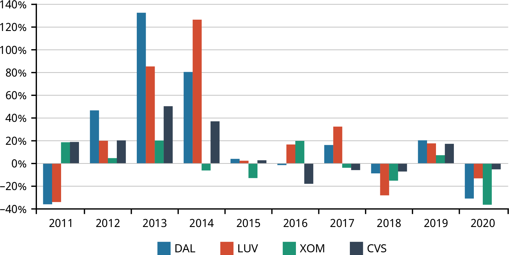
Figure 15.2 Yearly Returns for DAL, LUV, XOM, and CVS (data source: Yahoo! Finance)
Standard deviation is considered a measure of the risk of owning a stock. The larger the standard deviation of a stock’s annual returns, the further from the average that stock’s return is likely to be in any given year. In other words, the return for the stock is highly unpredictable. Although the return for CVS varies from year to year, it is not subject to the wide swings of the returns for DAL or LUV.
Why are stock returns so volatile? The value of the stock of a company changes as the expectations of the future revenues and expenses of the company change. These expectations may change due to a number of events and new information. Good news about a company will tend to result in an increase in the stock price. For example, DAL announcing that it will be opening new routes and flying to cities it has not previously serviced suggests that DAL will have more customers and more revenue in future years. Or if CVS announces that it has negotiated lower rent for many of its locations, investors will expect the expenses of the company to fall, leading to more profits. Those types of announcements will often be associated with a higher stock price. Conversely, if the pilots and flight attendants for DAL negotiate higher salaries, the expenses for DAL will increase, putting downward pressure on profits and the stock price.
LINK TO LEARNINGPeloton and RiskAn example of how news can impact the price of a stock occurred on May 5, 2021, when Peloton recalled all of its Tread+ and Tread products after the tragic death of a child and 70 injuries associated with use of its products.1 The previous day, Peloton stock traded for $96.70 per share. The stock price dropped approximately 15% when the recall was announced. The closing price for a share of Peloton on May 5 was$82.62.2 You can read the company’s statement about this recall (https://openstax.org/r/ the_companys_recall) online.
15.2
Risk and Return to Multiple Assets
Learning Outcomes
By the end of this section, you will be able to:
- Explain the benefits of diversification.
- Describe the relationship between risk and return for large portfolios.
- Compare firm-specific and systematic risk.
- Discuss how portfolio size impacts risk.
Diversification
So far, we have looked at the return and the volatility of an individual stock. Most investors, however, own shares of stock in multiple companies. This collection of stocks is known as a portfolio. Let’s explore why it is wise for investors to hold a portfolio of stocks rather than to pick just one favorite stock to own.
We saw that investors who owned DAL experienced an average annual return of 20.87% but also a large standard deviation of 51.16%. Investors who used all their funds to purchase DAL stock did exceptionally well during 2012–2014. But in 2020, those investors lost almost one-third of their money as COVID-19 caused a sharp reduction in air travel worldwide. To protect against these extreme outcomes, investors practice what is called diversification, or owning a variety of stocks in their portfolios.
Suppose, for example, you have saved $50,000 that you want to invest. If you purchased $50,000 of DAL stock, you would not be diversified. Your return would depend solely on the return on DAL stock. If, instead, you used
$5,000 to purchase DAL stock and used the remaining $45,000 to purchase nine other stocks, you would be diversifying. Your return would depend not only on DAL’s return but also on the returns of the other nine stocks in your portfolio. Investors practice diversification to manage risk.
It is akin to the saying “Don’t put all of your eggs in one basket.” If you place all of your eggs in one basket and that basket breaks, all of your eggs will fall and crack. If you spread your eggs out across a number of baskets, it is unlikely that all of the baskets will break and all of your eggs will crack. One basket may break, and you will lose the eggs in that basket, but you will still have your other eggs. The same idea holds true for investing. If you own stock in a company that does poorly, perhaps even goes out of business, you will lose the money you placed in that particular investment. However, with a diversified portfolio, you do not lose all your money because your money is spread out across a number of different companies.
- Trefis Team and Great Speculations. “Is Peloton’s Tread+ Recall an Opportunity to Buy the Stock?” Forbes, May 7, 2021. https://www.forbes.com/sites/greatspeculations/2021/05/07/is-pelotons-tread-recall-an-opportunity-to-buy-the-stock/
- Tomi Kilgore. “Peloton Stock Sinks to 8-Month Low after 125,000 Treadmills Recalled for ‘Risk of Injury or Death.’” MarketWatch. May 6, 2021. https://www.marketwatch.com/story/peloton-stock-sinks-toward-9-month-low-after-125-000-treadmills-recalled-for- risk-of-injury-or-death-11620233715
LINK TO LEARNINGDiversificationFidelity Investments Inc. is a multinational financial services firm and one of the largest asset managers in the world. In this educational video for investors (https://openstax.org/r/educational_investors), Fidelity provides an explanation of what diversification is and how it impacts an investor’s portfolio.
Table 15.7 shows the returns of investors who placed 50% of their money in DAL and the remaining 50% in LUV, XOM, or CVS. Notice that the standard deviation of returns is lower for the two-stock portfolios than for DAL as an individual investment.
|
|
|
|||
|
Year |
DAL |
DAL and LUV |
DAL and XOM |
DAL and CVS |
|
2011 |
−35.79% |
−34.86% |
−8.56% |
−8.43% |
|
2012 |
46.72% |
33.38% |
25.71% |
33.50% |
|
2013 |
132.61% |
109.00% |
76.36% |
91.50% |
|
2014 |
80.53% |
103.50% |
37.24% |
58.83% |
|
2015 |
4.05% |
3.24% |
−4.37% |
3.47% |
|
2016 |
−1.35% |
7.69% |
9.27% |
−9.59% |
|
2017 |
16.23% |
24.32% |
6.21% |
5.24% |
|
2018 |
−8.66% |
−18.47% |
−11.88% |
−7.85% |
|
2019 |
20.38% |
19.03% |
13.81% |
18.82% |
|
2020 |
−30.77% |
−21.90% |
−33.49% |
−17.95% |
|
Average |
22.40% |
22.49% |
11.03% |
16.75% |
|
Std Dev |
51.90% |
49.11% |
30.43% |
35.10% |
Table 15.7 Yearly Returns for DAL Versus a Two-Stock Portfolio Containing DAL and LUV, XOM, or CVS (data source: Yahoo! Finance)
As investors diversify their portfolios, the volatility of one particular stock becomes less important. XOM has good years with above-average returns and bad years with below-average (and even negative) returns, just like DAL. But the years in which those above-average and below-average returns occur are not always the same for the two companies. In 2014, for example, the return for DAL was greater than 80%, while the return for XOM was negative. On the other hand, in 2011, when DAL had a return of −35.15%, XOM had a positive return. When more than one stock is held, the gains in one stock can offset the losses in another stock, washing away some of the volatility.
When an investor holds only one stock, that one stock’s volatility contributes 100% to the portfolio’s volatility. When two stocks are held, the volatility of each stock contributes to the volatility of the portfolio. However, the volatility of the portfolio is not simply the average of the volatility of each stock held independently. How correlated the two stocks are, or how much they move together, will impact the volatility of the portfolio.
You will recall from our study of correlation in Regression Analysis in Finance that a correlation coefficient describes how two variables move relative to each other. A correlation coefficient of 1 means that there is a perfect, positive correlation between the two variables, while a correlation coefficient of −1 means that the two variables move exactly opposite of each other. Stocks that are in the same industry will tend to be more
strongly correlated than stocks that are in much different industries. During the 2011–2020 time period, the correlation coefficient for DAL and LUV was 0.87, the correlation coefficient for DAL and XOM was 0.35, and the correlation coefficient for DAL and CVS was 0.79. Combining stocks that are not perfectly positively correlated in a portfolio decreases risk.
Notice that investors who owned DAL and LUV from 2011 to 2020 would have had a lower portfolio standard deviation, but not much lower, than investors who just owned DAL. Because the correlation coefficient is less than one, the standard deviation fell. However, because the two stocks are in the same industry and exposed to many of the same economic issues, the correlation coefficient is relatively high, and combining those two stocks provides only a small decrease in risk.
This is because, as airlines, DAL and LUV face many of the same market conditions. In years when the economy is strong, the weather is good, fuel prices are low, and people are traveling a lot, both companies will do well. When something such as bad weather conditions reduces the amount of air travel for several weeks, both companies are harmed. By holding LUV in addition to DAL, investors can reduce exposure to risk that is specific to DAL (perhaps a problem that DAL has with its reservation system), but they do not reduce exposure to the risk associated with the airline industry (perhaps rising jet fuel prices). DAL and LUV tend to experience positive returns in the same years and negative returns in the same years.
On the other hand, investors who added XOM to their portfolio saw a significantly lower standard deviation than those who held just DAL. In years when jet fuel prices rise, harming the profits of both DAL and LUV, XOM is likely to see high profits. Diversifying a portfolio across firms that are less correlated will reduce the standard deviation of the portfolio more.
LINK TO LEARNINGHow to Build a Diversified PortfolioTV personality, former hedge fund manager, and author Jim Cramer encourages investors to build a diversified portfolio, having no more than 20% of a portfolio in one sector.3 Watch this CNBC video (https://openstax.org/r/CNBC_video) to learn more about how he suggests investors can build a diversified portfolio by purchasing five to 10 stocks.
Portfolio Size and Risk
As you add more stocks to a portfolio, the volatility, or standard deviation, of the portfolio decreases. The volatility of individual assets becomes less and less important. As we discussed earlier, the risk that is associated with events related to a particular company is called firm-specific risk, or unsystematic, risk. Examples of unsystematic risk would include a company facing a product liability lawsuit, a company inventing a new product, or accounting irregularities being detected. Holding a portfolio of stocks means that if one company you have invested in goes out of business because of poor management, you do not lose all your savings because some of your money is invested in other companies. Portfolio diversification protects you from being significantly impacted by unsystematic risk.
However, there is a level below which the portfolio risk does not drop, no matter how diversified the portfolio becomes. The risk that never goes away is known as systematic risk. Systematic risk is the risk of holding the market portfolio.
We have talked about reasons why a firm’s returns might be volatile; for example, the firm discovering a new technology or having a product liability lawsuit brought against it will impact that firm specifically. There are also events that broadly impact the stock market. Changes in the Federal Reserve Bank’s monetary policy and
- Abigail Stevenson. “Jim Cramer Shares His #1 Rule for Investing.” Make It. CNBC, March 15, 2016. https://www.cnbc.com/2016/03/ 03/cramer-forget-sectors-a-better-way-to-diversify.html
interest rates impact all companies. Geopolitical events, major storms, and pandemics can also impact the entire market. Investors in stocks cannot avoid this type of risk. This unavoidable risk is the systematic risk that investors in stocks have. This systematic risk cannot be eliminated through diversification.
In addition, as per research conducted by Meir Statman,4 the standard deviation of a portfolio drops quickly as the number of stocks in the portfolio increases from one to two or three (see Figure 2 illustration in this subsequent article by Statman (https://openstax.org/r/subsequent_Statman) for context). Increasing the size of the portfolio decreases the standard deviation, and thus the risk, of the portfolio. However, as the portfolio increases in size, the amount of risk reduced by adding one more stock to the portfolio will decrease. How many stocks does an investor need for a portfolio to be well-diversified? There is not an exact number that all financial managers agree on. A portfolio of 15 highly correlated stocks will offer less benefits of diversification than a portfolio of 10 stocks with lower correlation coefficients. A portfolio that consists of American Airlines, Spirit Airlines, United Airlines, Southwest Airlines, Delta Airlines, and Jet Blue, along with a few other stocks, is not very diversified because of the heavy concentration in the airline industry. The term diversified portfolio is a relative concept, but the average investor can create a reasonably diversified portfolio with approximately a dozen stocks.
15.3
The Capital Asset Pricing Model (CAPM)
Learning Outcomes
By the end of this section, you will be able to:
- Define risk premium.
- Explain the concept of beta.
- Compute the required return of a security using the CAPM.
Risk-Free Rate
The capital asset pricing model (CAPM) is a financial theory based on the idea that investors who are willing to hold stocks that have higher systematic risk should be rewarded more for taking on this market risk. The CAPM focuses on systematic risk, rather than a stock’s individual risk, because firm-specific risk can be eliminated through diversification.
Suppose that your grandparents have given you a gift of $20,000. After you graduate from college, you plan to work for a few years and then apply to law school. You want to use the $20,000 your grandparents gave you to pay for part of your law school tuition. It will be several years before you are ready to spend the money, and you want to keep the money safe. At the same time, you would like to invest the money and have it grow until you are ready to start law school.
Although you would like to earn a return on the money so that you have more than $20,000 by the time you start law school, your primary objective is to keep the money safe. You are looking for a risk-free investment. Lending money to the US government is considered the lowest-risk investment that you can make. You can purchase a US Treasury security. The chances of the US government not paying its debts is close to zero.
Although, in theory, no investment is 100% risk-free, investing in US government securities is generally considered a risk-free investment because the risk is so miniscule.
- Meir Statman. “How Many Stocks Make a Diversified Portfolio?” Journal of Financial and Quantitative Analysis 22, no. 3 (September 1987): 353–363. https://doi.org/10.2307/2330969
The rate that you can earn by purchasing US Treasury securities is a proxy for the risk-free rate. It is used as an investing benchmark. The average rate of return for the three-month US Treasury security from 1928 to 2020 is 3.36%.5 You can see that you will not become immensely wealthy by investing in US Treasury bills.
Another characteristic of US Treasury securities, however, is that their volatility tends to be much lower than that of stocks. In fact, the standard deviation of returns for the US Treasury bills is 3.0%. Unlike the returns for
stocks, the return on US Treasury bills has never been negative. The lowest annual return was 0.03%, which occurred in 2014.6
LINK TO LEARNINGUS Treasury SecuritiesVisit the website of the US Department of the Treasury (https://openstax.org/r/home.treasury) to learn more about US Treasury securities. You will find current interest rates for both short-term securities (US Treasury bills) and long-term securities (US Treasury bonds).
Risk Premium
You know that if you use your $20,000 to invest in stock rather than in US Treasury bills, the outcome of the investment will be uncertain. Your investments may do well, but there is also a risk of losing money. You will only be willing to take on this risk if you are rewarded for doing so. In other words, you will only be willing to take the risk of investing in stocks if you think that doing so will make you more than you would make investing in US Treasury securities.
From 1928 to 2020, the average return for the S&P 500 stock index has been 11.64%, which is much higher than the 3.36% average return for US Treasury bills.7 Stock returns, with a standard deviation of 19.49%, however, have also been much more volatile. In fact, there were 25 years in which the return for the S&P 500 index was negative.
You may not be willing to take the risk of losing some of the money your grandparents gave you because you have been setting it aside for law school. If that’s the case, you will want to invest in US Treasury securities.
You may have money that you are saving for other long-term goals, such as retirement, with which you are willing to take some risk. The extra return that you will earn for taking on risk is known as the risk premium. The risk premium can be thought of as your reward for being willing to bear risk.
The risk premium is calculated as the difference between the return you receive for taking on risk and what you would have returned if you did not take on risk. Using the average return of the S&P 500 (to measure what investors who bear the risk earn) and the US Treasury bill rate (to measure what investors who do not bear risk earn), the risk premium is calculated as


Beta
The risk premium represents how much an investor who takes on the market portfolio is rewarded for risk. Investors who purchase one stock—DAL, for example—experience volatility, which is measured by the standard deviation of that stock’s returns. Remember that some of that volatility, the volatility caused by firm- specific risk, can be diversified away. Because investors can eliminate firm-specific risk through diversification, they will not be rewarded for that risk. Investors are rewarded for the amount of systematic risk they incur.
- “Historical Return on Stocks, Bonds and Bills: 1928–2020.” Damodaran Online. Stern School of Business, New York University, January 2021. http://pages.stern.nyu.edu/~adamodar/New_Home_Page/datafile/histretSP.html
- Ibid.
- Ibid.
Interpreting Beta
The relevant risk for investors is the systematic risk they incur. The systematic risk of a particular stock is measured by how much the stock moves with the market. The measure of how much a stock moves with the market is known as its beta. A stock that tends to move in sync with the market will have a beta of 1. For these stocks, if the market goes up 10%, the stock generally also goes up 10%; if the market goes down 5%, stocks with a beta of 1 also tend to go down 5%.
If a company has a beta greater than 1, then the stock tends to have a more pronounced move in the same direction as a market move. For example, if a stock has a beta of 2, the stock will tend to increase by 20% when the market goes up by 10%. If the market falls by 5%, that same stock will tend to fall by twice as much, or 10%. Thus, stocks with a beta greater than 1 experience greater swings than the overall market and are considered to be riskier than the average stock.
On the other hand, stocks with a beta less than 1 experience smaller swings than the overall market. A beta of 0.5, for example, means that a stock tends to experience moves that are only 50% of overall market moves. So, if the market increases by 10%, a stock with a beta of 0.5 would tend to rise by only 5%. A market decline of 5% would tend to be associated with a 2.5% decrease in the stock.
Calculating Betas
The calculation of beta for DAL is demonstrated in Figure 15.3. Monthly returns for DAL and for the S&P 500 are plotted in the diagram. Each dot in the scatter plot corresponds to a month from 2018 to 2020; for example, the dot that lies furthest in the upper right-hand corner represents November 2020. The return for the S&P 500 was 10.88% that month; this return is plotted along the horizontal axis. The return for DAL during November 2020 was 31.36%; this return is plotted along the vertical axis.
You can see that generally, when the overall stock market as measured by the S&P 500 is positive, the return for DAL is also positive. Likewise, in months in which the return for the S&P 500 is negative, the return for DAL is also usually negative. Drawing a line that best fits the data, also known as a regression line, summarizes the relationship between the returns for DAL and the S&P 500. The slope of this line, 1.39, is DAL’s beta. Beta measures the amount of systematic risk that DAL has.
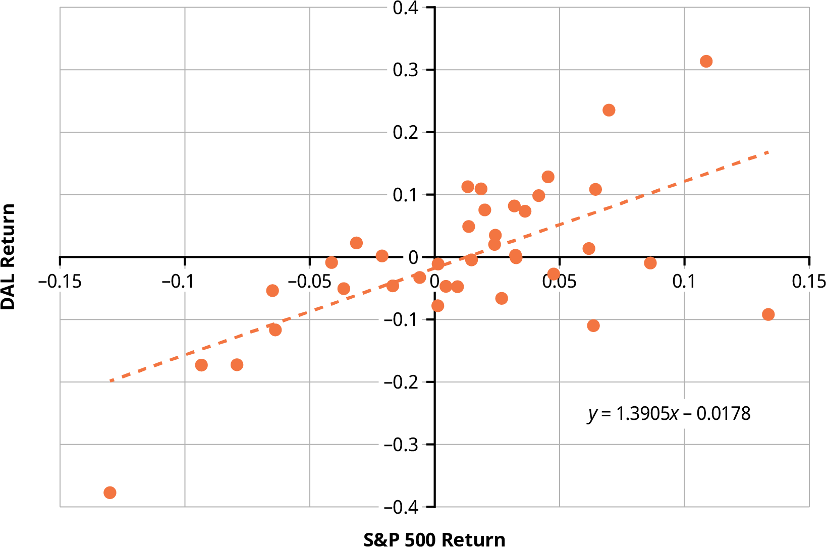
Figure 15.3 Calculation of Beta for DAL (data source: Yahoo! Finance)
CAPM Equation
Because DAL’s beta of 1.39 is greater than 1, DAL is riskier than the average stock in the market. Finance theory suggests that investors who purchase DAL will expect a higher rate of return to compensate them for this risk. DAL has 139% of the average stock’s systematic risk; therefore, investors in the stock should receive 139% of the market risk premium.

The capital asset pricing model (CAPM) equation is


where Re is the expected return of the asset, Rf is the risk-free rate of return, and Rm is the expected return of the market. Given the average S&P 500 return of 11.64% and the average US Treasury bill return of 3.36%, the expected return of DAL would be calculated as

LINK TO LEARNINGCalculating BetaMany providers of stock data and investment information will list a company’s beta. Two internet sources that can be used to find a company’s beta are Yahoo! Finance (https://openstax.org/r/finance.yahoo) and MarketWatch (https://openstax.org/r/marketwatch_search). Various sources may not provide the exact same value for beta for a company. For example, in early February 2021, Yahoo! Finance reported that the beta for DAL was 1.46,8 while MarketWatch reported it as 1.29.9 Both of these numbers are slightly different from the 1.39 calculated in the graph above.There are several reasons why beta may vary slightly from source to source. One is the time frame used in the beta calculation. Data from three years were used to calculate the beta in Figure 15.3. Time frames ranging from three to five years are commonly used when calculating beta. Another reason different sources might report different betas is the frequency with which the data is collected. Monthly returns are used in Figure 15.3; some analysts will use weekly data. Finally, the S&P 500 is used to measure the market return in Figure 15.3; the S&P 500 is one of the most common measures of overall market returns, but alternatives exist and are used by some analysts
LINK TO LEARNINGCAPMWatch this video (https://openstax.org/r/pricing-model-capm) for further information about the CAPM.
- “Delta Air Lines, Inc. (DAL).” Yahoo! Finance. Verizon Media, accessed February 2021. https://finance.yahoo.com/quote/DAL/
- “Delta Air Lines Inc.” MarketWatch. Accessed February 2021. https://www.marketwatch.com/investing/stock/dal
15.4
Applications in Performance Measurement
Learning Outcomes
By the end of this section, you will be able to:
Sharpe Ratio
Investors want a measure of how good a professional money manager is before they entrust their hard- earned funds to that professional for investing. Suppose that you see an advertisement in which McKinley Investment Management claims that the portfolios of its clients have an average return of 20% per year. You know that this average annual return is meaningless without also knowing something about the riskiness of the firm’s strategy. In this section, we consider some ways to evaluate the riskiness of an investment strategy.
A basic measure of investment performance that includes an adjustment for risk is the Sharpe ratio. The Sharpe ratio is computed as a portfolio’s risk premium divided by the standard deviation of the portfolio’s return, using the formula


The portfolio risk premium is the portfolio return RP minus the risk-free return Rf; this is the basic reward for bearing risk. If the risk-free return is 3%, McKinley Investment Management’s clients who are earning 20% on their portfolios have an excess return of 17%.
 The standard deviation of the portfolio’s return,, is a measure of risk. Although you see that McKinley’s clients earn a nice 20% return on average, you find that the returns are highly volatile. In some years, the clients earn much more than 20%, and in other years, the return is much lower, even negative. That volatility leads to a standard deviation of returns of 26%. The Sharpe ratio would be
  , or 0.65.
Thus, the Sharpe ratio can be thought of as a reward-to-risk ratio. The standard deviation in the denominator can be thought of as the units of risk the investor has. The numerator is the reward the investor is receiving for taking on that risk.
LINK TO LEARNINGSharpe RatioThe Sharpe ratio was developed by Nobel laureate William F. Sharpe. You can visit Sharpe’s Stanford University website (https://openstax.org/r/stanford_wfsharpe) to find videos in which he discusses financial topics and links to his research as well as his advice on how to invest.
Treynor Measurement of Performance
Another reward-to-risk ratio measurement of investment performance is the Treynor ratio. The Treynor ratio is calculated as


Just as with the Sharpe ratio, the numerator of the Treynor ratio is a portfolio’s risk premium; the difference is that the Treynor ratio focus focuses on systematic risk, using the beta of the portfolio in the denominator, while the Shape ratio focuses on total risk, using the standard deviation of the portfolio’s returns in the
denominator.

If McKinley Investment Management has a portfolio with a 20% return over the past five years, with a beta of

1.2 and a risk-free rate of 3%, the Treynor ratio would be
Both the Sharpe and Treynor ratios are relative measures of investment performance, meaning that there is not an absolute number that indicates whether an investment performance is good or bad. An investment manager’s performance must be considered in relation to that of other managers or to a benchmark index.
Jensen’s Alpha
Jensen’s alpha is another common measure of investment performance. It is computed as the raw portfolio return minus the expected portfolio return predicted by the CAPM:


Suppose that the average market return has been 12%. What would Jensen’s alpha be for McKinley Investment Management’s portfolio with a 20% average return and a beta of 1.2?


Unlike the Sharpe and Treynor ratios, which are meaningful in a relative sense, Jensen’s alpha is meaningful in an absolute sense. An alpha of 0.062 indicates that the McKinley Investment Management portfolio provided a return that was 6.2% higher than would be expected given the riskiness of the portfolio. A positive alpha indicates that the portfolio had an abnormal return. If Jensen’s alpha equals zero, the portfolio return was exactly what was expected given the riskiness of the portfolio as measured by beta.

THINK IT THROUGH
Comparing the Returns and Risks of Portfolios
You are interviewing two investment managers. Mr. Wong shows that the average return on his portfolio for the past 10 years has been 14%, with a standard deviation of 8% and a beta of 1.2. Ms. Petrov shows that the average return on her portfolio for the past 10 years has been 16%, with a standard deviation of 10% and a beta of 1.6. You know that over the past 10 years, the US Treasury security rate has averaged 2% and the return on the S&P 500 has averaged 11%. Which portfolio manager do you think has done the better job?
Solution:
The Sharpe ratio for Mr. Wong’s portfolio is, and the Treynor ratio is. The Sharpe ratio for Ms. Petrov’s portfolio is, and the Treynor ratio is.
Jensen’s alpha for Mr. Wong’s portfolio is
Jensen’s alpha for Ms. Petrov’s portfolio is
All three measures of portfolio performance suggest that Mr. Wong’s portfolio has performed better than Ms. Petrov’s has. Although Ms. Petrov has had a larger average return, the portfolio she manages is riskier. Ms. Petrov’s portfolio is more volatile than Mr. Wong’s, resulting in a higher standard deviation. Ms.
Petrov’s portfolio has a higher beta, which means it has a higher amount of systematic risk. The CAPM suggests that a portfolio with a beta of 1.6 should have an expected return of 16.4%. Because Ms. Petrov’s
portfolio has an average return of less than that, investors in Ms. Petrov’s portfolio are not rewarded for the risk that they have taken as much as would be expected.
15.5
Using Excel to Make Investment Decisions
Learning Outcomes
By the end of this section, you will be able to:
- Calculate the average return and standard deviation for a stock.
- Calculate the average return and standard deviation for a portfolio.
- Calculate the beta of a stock.
Average Return and Standard Deviation for a Single Stock
Excel can be used to calculate the average returns and the standard deviation of returns for both a single stock and a portfolio of stocks. It can also be used to calculate the beta for a stock. Historic stock price data for stocks you are interested in analyzing can easily be downloaded from sites such as Yahoo! Finance into Excel. The examples in this section use monthly stock data from December 2017 to December 2020 from Yahoo!
Finance.
Monthly price data for AMZN (Amazon) is shown in column B of Figure 15.4. To begin, monthly returns must be calculated from the price data using the formula
The ending prices shown in Figure 15.4 are the last price the stock traded for each month. Each month, the return is calculated under the assumption that you purchased the stock at the last trading price of the previous month and sold at the last price of the current month. Thus, the return for January 2018 is calculated as


 This is accomplished in Excel by placing the formula =(B3-B2)/B2 in cell C3. This formula can then be copied down the spreadsheet through row C38. Now that each monthly return is in column C, you can calculate the average of the monthly returns in cell C39 and the standard deviation of returns in cell C40.
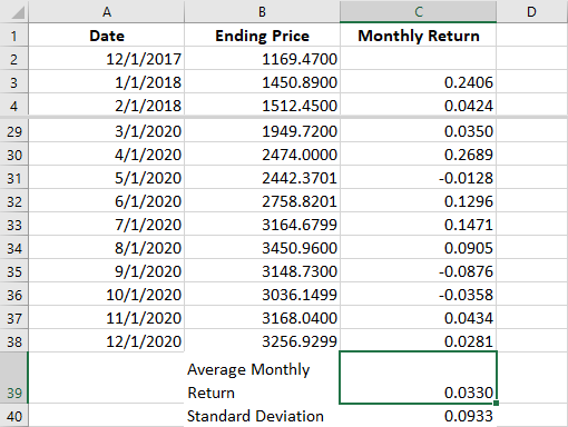
Figure 15.4 Calculating the Average Return and the Standard Deviation of Returns for AMZN (data source: Yahoo! Finance)
Over the three-year period, the average monthly return for AMZN was 3.3%. However, this return was highly volatile, with a standard deviation of 9.33%. Remember that this means that approximately two-thirds of the time, the monthly return from AMZN was between −6.03% and 12.63%.

Download the spreadsheet file (https://openstax.org/r/google_spread_sheet) containing key Chapter 15 Excel exhibits.
Average Return and Standard Deviation for a Portfolio
The Excel screenshot in Figure 15.5 shows the return and standard deviation calculation for a portfolio. This sample four-stock portfolio contains AMZN, CVS, AAPL (Apple), and NFLX (Netflix). This portfolio is constructed as an equally weighted portfolio; because there are four stocks in this portfolio, each has a weight of 25%.
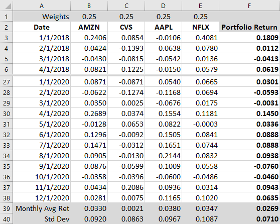
Figure 15.5 Calculation of the Average Return and Standard Deviation for a Portfolio (data source: Yahoo! Finance)
The monthly returns for each stock are recorded in their respective columns. The portfolio return for each month is calculated as the weighted average of the four monthly individual stock returns. The formula for the portfolio return is


The formula =$B$1*B3+$C$1*C3+$D$1*D3+$E$1*E3 is placed in cell F3. The formula is then copied down column F to calculate the portfolio return for each month. After the monthly portfolio return is calculated, then the average monthly portfolio return is calculated in cell F39. The average monthly portfolio return is 2.69%.

 Because this is an equally weighted portfolio, with each of the four stocks impacting the portfolio return in the same way, the average monthly portfolio return of 2.69% is the same as the sum of the average monthly returns of the four stocks divided by four, or
  .
.
The standard deviation of the monthly portfolio returns is calculated in cell F40. This four-stock portfolio has a standard deviation of 7.10%. Unlike the average return, this standard deviation is not equal to the average of the standard deviations of returns of the four stocks. In fact, the standard deviation for the portfolio is less than the standard deviation for any one of the four stocks. Remember that this occurs because the stock returns are not perfectly positively correlated. The high return of one of the stocks in one month is dampened by a lower return in another stock during the same month. Likewise, a negative return in one stock during a month might be offset by a positive return in one of the other three stocks during the same month. This is the risk reduction benefit of holding a portfolio of stocks.
Calculating Beta
The standard deviation of a stock’s returns indicates the stock’s volatility. Remember that the volatility is caused by both firm-specific and systematic risk. Investors will not be rewarded for firm-specific risk because
they can diversify away from it. Investors are, however, rewarded for systematic risk. To determine how much of a firm’s risk is due to systematic risk, you can use Excel to calculate the stock’s beta.
To calculate a stock’s beta, you need the monthly return for the market in addition to the monthly market return for the stock. In column B in Figure 15.6, the monthly return for SPY, the SPDR S&P 500 Trust, is recorded. SPY is an ETF that was created to mimic the performance of the S&P 500 index by State Street Global Advisors and is often used as a proxy for the overall market performance. The monthly returns for AMZN are visible in column C. It is important that these returns be lined up so that the returns for a particular month for both securities appear in the same row number. Also, you want to place the returns for SPY in the column to the left of the returns for AMZN so that when you create your graph, SPY will automatically appear on the horizontal axis.
LINK TO LEARNINGState Street Global AdvisorsYou can learn more about State Street Global Advisors and its creation of the first ETF by visiting the company’s history page at its website (ssga.com) (https://openstax.org/r/ssga_institutional_our-history).
You will use a scatter plot to create a graph. In Excel, go to the Insert tab, and then from the Chart menu, choose the first scatter plot option.
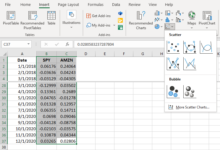
Figure 15.6 Excel Format for Calculating Beta (data source: Yahoo! Finance)
Selecting the scatter plot option will result in a chart being inserted that looks like the chart in Figure 15.7. Each dot represents one month’s combination of returns, with the return for SPY measured on the horizontal axis and the return for AMZN measured on the vertical axis. Consider, for example, the dot in the furthest upper right-hand section of the figure. This dot is the plot of returns for the month of April 2020, when the return for SPY was 13.36% (measured on the horizontal axis) and the return for AMZN was 26.89% (measured on the
vertical axis).
Hover your mouse over one of the dots, and right-click the dot to pull up a chart formatting menu. This menu will allow you to add labels to your axis and polish your chart in additional ways if you would like. Select the option Add Trendline.
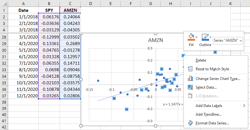
Figure 15.7 Creating a Scatter Plot in Excel (data source: Yahoo! Finance)


When the trendline is inserted, a formatting box will appear on the right of your screen (see Figure 15.8). If it is not already selected, choose the Linear trendline option. Scroll down and select the “Display Equation on chart” option. You will see the equationappear on the screen. This is the equation for the best-fit line that shows how AMZN moves when the market moves. The slope of this line, 1.1477, is the beta for AMZN. This tells you that for every 10% move the overall market makes, AMZN tends to move 11.477%. Because AMZN tends to move a little more than the broader market, it has a little more systematic risk than the average stock in the market.
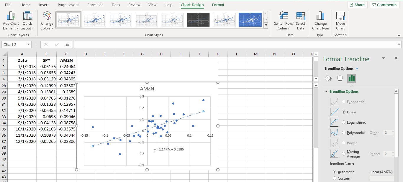
Figure 15.8 Inserting a Trendline to Determine Beta (data source: Yahoo! Finance)
 Summary
Risk and Return to an Individual Asset
Investors are interested in both the return they can expect to receive when making an investment and the risk associated with that investment. In finance, risk is considered the volatility of the return from time period to time period. Historical returns are measured by the arithmetic average, and the risk is measured by the standard deviation of returns.
Risk and Return to Multiple Assets
As investors hold multiple assets in a portfolio, they are able to eliminate firm-specific risk. However, systematic or market risk remains, even if an investor holds the market portfolio. The return to a portfolio is measured by the arithmetic average, and the risk is measured by the standard deviation of the returns of the portfolio. The risk of the portfolio will be lower than the weighted average of the risk of the individual securities because the returns of the securities are not perfectly correlated. A low or negative return for one stock in a period can be offset by a high return for another stock in the same period.
The Capital Asset Pricing Model (CAPM)
The capital asset pricing model (CAPM) relates the expected return of an asset to the systematic risk of that asset. Investors will be rewarded for taking on systematic risk. They will not be rewarded for taking on firm- specific risk, however, because that risk can be diversified away.
Applications in Performance Measurement
Because investors are not simply interested in returns but are also interested in risk, the success of a portfolio cannot be measured simply by considering the portfolio’s return. In order to compare investment portfolios, risk and return must both be taken into consideration. The Sharpe ratio and the Treynor ratio are two measures that provide a reward-to-risk measure of a portfolio. Jensen’s alpha provides a measure of the abnormal return of a portfolio, considering the portfolio’s risk level.
Using Excel to Make Investment Decisions
Using Excel to manipulate publicly available stock data makes calculating the average return of a stock and the standard deviation of returns easy. The average return for a portfolio and the standard deviation of the portfolio returns can also be calculated easily. By comparing the returns of a stock with the returns of the overall market using Excel charting tools, the beta for a stock, which measures systematic risk, can be determined.
 Key Terms
arithmetic average return the sum of an asset’s annual returns over a number of years divided by the number of years
beta a measure of how a stock moves relative to the market
capital asset pricing model (CAPM) the expected return of a security, equal to the risk-free rate plus a premium for the amount of risk taken
capital gain yield the difference between the price a stock is sold for and the price that was originally paid for it divided by the price originally paid
diversification holding a variety of assets in a portfolio
dividend yield the total dividends received by the owner of a share of stock divided by the price originally paid for the stock
effective annual rate (EAR) returns expressed on an annualized or yearly basis; allows for the comparison of various investments
firm-specific risk the risk that an event may impact the expected revenue or costs of a firm, thereby
impacting the returns to investors; also known as diversifiable risk
geometric average return the compound annual return derived from the effective annual rate and time value of money formulas
holding period percentage return the gain received from holding a stock, calculated by adding the amount received when the stock is sold to any dividends earned while holding the stock, subtracting the price originally paid for the stock, then dividing the difference by the price originally paid
Jensen’s alpha a measure of portfolio performance, calculated as the raw portfolio return minus the expected portfolio return predicted by the CAPM
market risk premium the reward for taking on the average amount of market risk
portfolio a collection of owned stocks
realized return the total return of an investment that occurs over a particular time period
risk premium the extra return earned by taking on risk
risk-free rate the reward for lending money when there is no risk of not receiving the principal and interest as promised
Sharpe ratio a reward-to-risk measure of portfolio performance, calculated by subtracting the risk-free rate from the average portfolio return and then dividing by the standard deviation of the portfolio
systematic risk risk that impacts the entire market and cannot be diversified away; also known as market risk
Treynor ratio a reward-to-risk measure of portfolio performance, calculated by subtracting the risk-free rate from the average portfolio return and then dividing by the beta of the portfolio